Evidence for a Geodynamo Driven by Thermal Energy in the Outermost Core and by Precession Deeper in the Outer Core

Fuller MD

International Journal of Earth Science and Geophysics

Evidence for a Geodynamo Driven by Thermal Energy in the Outermost Core and by Precession Deeper in the Outer Core

Michael D Fuller^*

Department of Earth Science, University of California at Santa Barbara, California, USA

^*Corresponding author

Michael D Fuller, Professor Emeritus, Department of Earth Science, University of California at Santa Barbara, Santa Barbara, California, 93106, USA, E-mail: [email protected]

Int J Earth Sci Geophys, ijesg-3-012, (Volume 3, Issue 1), Research Article

Received: May 18, 2017
Accepted: August 30, 2017
Published: September 02, 2017

Citation: Fuller MD (2017) Evidence for a Geodynamo Driven by Thermal Energy in the Outermost Core and by Precession Deeper in the Outer Core. Int J Earth Sci Geophys 3:012.

Copyright: © 2017 Fuller MD. This is an open-access article distributed under the terms of the Creative Commons Attribution License, which permits unrestricted use, distribution, and reproduction in any medium, provided the original author and source are credited.

Abstract

VGP (Virtual Geomagnetic Pole) paths during reversals are preferentially located in roughly north south circum-Pacific arcs, where the temperature of the mantle at the core mantle boundary is lowest. This indicates that the movement of magnetic flux concentrations in the outermost core responds to thermal constraints during the reversal. Hence thermal energy plays a role in driving the geodynamo. The preponderance of the occurrence of reversals when the obliquity is lower than the average within the last 5 Ma and their preferential onset during the decreasing half of the obliquity cycle provide evidence for a role of precession in driving the dynamo. The geodynamo therefore appears to involve a combination of thermal and precessional energy. A reversal with its decay of the dipole intensity by almost an order of magnitude, the polarity switch, and regrowth of the new axial dipole involves an intermediate equatorial field source, whose polarity also switches with the axial dipole. The whole reversal process for each of the last two reversals falls within approximately one obliquity cycle of 41,000 years and the polarity switch is close to the midpoint of the cycle.

Introduction

It has long been held that thermal convection, or the rise of low density material released in the formation of the inner core, determine the motion of the fluid outer core and hence drive the geodynamo [1,2]. Here independent evidence of the role of thermal energy in constraining the outermost core flow during reversals is presented. Precession is less commonly held to play a role in the geodynamo, but has a long history stretching back to the classic studies of Poincaré [3]. Evidence is also given here for precession energy contributing to driving the dynamo. Finally, a model based upon the combined effect of convection and precession, as the energy source of the geodynamo has already been proposed and suggests that neither source is adequate to drive the geodynamo alone [4].

Thermal Constraints on Reversal VGP Paths

Paleomagnetic reversal records are largely consistent with the controversial suggestion made first by Clement and Kent [5] that VGP paths during reversals preferentially follow on the one hand the longitudes of the Americas and the Eastern Pacific, and on the other of East Asia and the Western Pacific: they are therefore predominantly circum-Pacific. The authors demonstrated this by first plotting the latitudes and longitudes of transitional VGPs and then showing the distribution of VGPs, as a function of longitude. In addition, Hoffman and Singer [6] reported concentrations of VGP's at particular latitudes within these longitudes for a number of reversals, demonstrating that it was a relatively long term aspect of the field. Laj, et al. [7] plotted the raw VGP paths and noted the occurrence at the same preferred longitudes of VGP paths during reversals of (1) The strongest non-dipole field features (Figure 1a), (2) Longitudinal flow in the outermost core (Figure 1b), and (3) Anomalous mantle P-wave velocities in the lowermost mantle (Figure 1c) showing that these longitudes have special geophysical significance. The P-wave velocity anomaly is particularly important because it indicates that the mantle is at lower temperatures there than elsewhere on the core mantle boundary. This shows that the pattern of outermost core flow responds to thermal constraints.

Given such a flow pattern, could it play a role in determining the VGP paths during reversals? If there were a dominant radial inward flux feature during reversals, as appears to be the case in some field models [8,9], then optimum routes are evident for such a feature to bring about a reversal of the flux polarity in the outermost fluid core (Figure 1b). For example, in an R-N transition the south geographic pole inward flux could move away from the pole over SE Asia, turn to follow westward near equatorial flow, and finally turn north over N. America. An N-R reversal path would be simpler, the north geographic inward polar flux could move southward over East Asia, and continue south to the east of S. Africa. Excursions can be equally well accommodated. Beginning from a reversed field configuration, the inward flux would behave as in an R-N reversal, but after motion along the equatorial flow, it would follow the return flow to its original location instead of turning north to give the reversal. It does then appear that the outermost core flow could play a role in reversals and excursions, in addition to revealing the thermal constraints on the reversal process.

There are two special regions in the outermost core flow pattern. One is where the flows within the longitudinal bands are convergent to the equator in the equatorial Indian Ocean, and another is in equatorial South America, where they are divergent from the equator (Figure 1b). The site in the Indian Ocean is also the site of the maximum increase in the vertical component in the present field and part of the main southern hemisphere non-dipole anomaly (Figure 1a). Strong westward equatorial flow links this region to the second special site in equatorial South America. This second site is also the region of maximum decrease of the vertical component in the present field. Unlike the SE Asian site, this region in South America is not part of the main southern hemisphere outward non-dipole anomaly, but appears to interrupt it with a relatively weak inward non-dipole source. Evidently these non-dipole sources are important in the outermost core flow pattern and in the present field, as well as during recent reversal transitions. The East Asian and South American sites and are possible sites for upwelling and down welling of core fluid carrying magnetic field flux. Moreover, both the SE Asian and South American site each give rise to a single inward non-axial field source in the equatorial plane dominating the reversal immediately before and after the polarity switch.

The SE Asian location is similar to regions where concentrations of VGP's were found to occur during a number of reversals by Hoffman and Singer [6], so as noted above it appears to be a relatively long term feature of the field. These two special sites are also the locations of the precursor and rebound sites described by Valet, et al. [10] and it is towards them that the VGP paths move before and after the midpoint of the reversal. This is seen particularly clearly in the beautiful drift sediment records of the reversal at the top of the Jaramillo (N-R) of Channell and colleagues [11], shown in Figure 2a and Figure 2c. These phenomena again imply relatively long term aspects of the flow pattern we see today.

From these records and those from intrusions [12], it is clear that the VGP paths are enhanced secular variation loops immediately before and after the actual polarity switch, when the axial dipole is weakest. After the precursor in the N-R reversal, high latitude northerly poles are briefly seen again before the polarity switch gets underway, revealing that a normal dipole field component is still present, although weakened, at this stage of the reversal. After the midpoint of the switch and before the rebound, high latitude southerly poles are seen, indicating the presence of a reversed dipole moment already at this point. Similarly in the R-N reversals, high latitude reversed poles are seen after the precursor and before the polarity switch. Evidently a key factor in determining these VGP paths during the reversal is the greater strength of the precursor and rebound sources compared with the axial dipole near to the midpoint of the reversal. In complete contrast, when the field is not reversing and the axial dipole is dominant much smaller, more familiar smaller secular variation loops of the VGP are seen at high latitudes.

There are indications in the VGP paths of the last two reversals that the precursor of an N-R reversal becomes the rebound of an R-N reversal and vice versa [11], although the Brunhes-Matuyama (BM) R-N reversal does not show comparably strong precursor and rebounds to those of the N-R of the Matuyama-Jaramillo (MJ) reversal. In addition, equally well documented VGP paths for the R-N Brunhes-Matuyama (BM) reversal from similar sections give very different records, with a convoluted path for the polarity switch in this R-N reversal in contrast to the relatively simple switch in the N-R Matuyama-Jaramillo (MJ) reversal (Figure 2a and Figure 2c).

Although the VGP paths for these last two reversals in earth history are profoundly different, they both have clear relations to the present outermost core flow pattern, whether they are compared with the version in Figure 1b or Figure 2b. In the N-R (MJ) polarity switch the VGP moves from north to south over East Asia following a relatively continuous favorable flow toward the south passing the southern tip of Africa. In contrast in the R-N (BM) polarity switch, when the VGP path and hence the inward flux source reaches the equator, the dominant flow path is to the west and there is no obvious direct flow path to the north. This path has sequences with progressive small incremental changes, similar to the N-R reversal, but there are also major discontinuous changes, the strongest of which takes the VGP from Central Asia to the tip of South Africa. After further small changes parallel to the dominant equatorial flow path, the VGP path moves rapidly to the north.

To summarize: that the outermost core flow pattern can explain these two very different reversal records by the effect of regions of favorable and unfavorable flow for the dominant flux concentrations during the reversal. This tells us that thermal energy is not only involved in driving the dynamo, but that it appears to play a direct role in the reversal process. The VGP construction appears to be tracking sites of dominant inward radial flux, which are following the outermost core flow.

Evidence for a Role of Precession in Driving the Geodynamo

There have long been essentially two basic types of dynamo models. One is dependent upon thermal effects such as convection, or the rise of low density material coming from the formation of the inner core. The only other commonly considered feasible mechanisms to generate motion in the outer core are related to orbital motions, such as precession, and their effect on the fluid outer core. Turning from thermally controlled aspects of the geodynamo to precession, if precession energy contributes to driving the geodynamo, it would likely be sensitive to the orbital parameters of Earth's rotation axis, such as obliquity and orbital eccentricity. It has been suggested that there is evidence in the geomagnetic field history for the 100,000 year periodicity of orbital eccentricity [14]. A further simple test of a possible role of precession in driving the dynamo is to compare the histories of the geomagnetic field and the obliquity, using the calculations of the obliquity by Laskar [15].

One such test would be to compare the standard intensity record of the recent field [16] with the variation in obliquity. This yields some interesting correlated features [17,18], but as Xuang and Channell [19] have demonstrated the details of the intensity record may have been degraded by variations in the magnetic properties of sediments downcore, which influence the intensity estimates obtained by standard normalization techniques, although whether this alone can account for the correlation seen between recent major changes in geomagnetic field history and the obliquity is not clear.

A second test, which avoids the difficulty of involving intensity estimates, is to compare the occurrence of reversals with the history of the obliquity (Figure 3a). When the comparison is made between an average value of the maximum of the obliquity over an extended time interval (Figure 3b), this has the additional benefit of being less sensitive to the accuracy of the age determinations of the reversals. If the obliquity plays no role in the occurrence of reversals, there should be as many reversals when the obliquity is above the average value as when it is below. Figure 3a shows the result of a comparison between the occurrence of individual reversals and the raw obliquity signal, while Figure 3b gives a comparison of their occurrence with a 5-point running average of the maximum obliquity values. If we compare these data for the last 5 Ma, we find that whereas 4 reversals took place when the obliquity parameter is above the average value of ~24°, 13 took place when it is below 24°. An even more intriguing aspect of the distribution in Figure 3b is that 9 of the 17 reversals fall within the overall obliquity low between 3.0 and 4.7 Ma, when the obliquity is consistently below the mean [20].

If we compare the various times when the averaged obliquity parameter falls below the mean, we find that the two most recent such intervals lasted about half a million years and 2 reversals took place in each, whereas during the intervening highs only 1 reversal took place. The behavior of the field is very different during the earlier extended low obliquity interval, lasting ~1.7 Ma. The comparison between the occurrence of reversals and extremes of the chosen obliquity parameter is even more remarkable. When it is more than 0.2° greater than the mean there is 1 reversal in 5 Ma, whereas when it is more than 0.2° lower than the mean there are a total of 7 reversals, with 4 between ~3.0 and 3.5 Ma and 3 between ~4.0 and 4.5. Within the last 5 Ma, when the obliquity parameter is more than 0.2° lower than the mean, there are then 7 reversals, but only 1 when it is more than 0.2° higher than the mean. This suggests that the dynamo was in a less stable polarity state for a period of ~1.7 Ma, when the obliquity was low and that during this time it was more prone to reverse. Thus the effect of precession is seen in the history of the geomagnetic field for the last 5 Ma and so precession appears to be involved in driving the geodynamo.

Another way in which a possible effect of precession might be seen in the history of the geomagnetic field is to check for a correlation between the onset of reversals and the phase in the obliquity cycles. This test is more difficult because of the requirement to know the timing of reversal onsets very accurately and is only practical for the most recent reversals. Nevertheless it was found that that there is a preference for the onset to occur during the half cycle of the decrease of the obliquity from its maximum value in the well dated last reversal, during the previous two, and for reversals between 2.5 and 3.4 Ma [18], although the possibility that such a relationship may extend further back in time has been challenged [21]. Continuing to consider the past 5 Ma, there have been many obliquity cycles, but only rarely did the major decrease in intensity and the onset of a reversal take place, so that there must be an additional as yet unknown trigger for reversals to occur besides the magnitude of the obliquity.

Two other possible tests for a role of precession in driving the dynamo come from the onset and length of excursions. Like true reversals they too tend to begin during the decrease of the obliquity from its maximum. They also tend to have total lengths, which fall within a single cycle of the obliquity signal [18], but these suggestions are more difficult to document than the preponderance of reversal occurrences with obliquity lows and the timing of their onset with the phase of the obliquity signal and are as yet less convincing.

To summarize, there are a number of indications that precession may play a role in the geodynamo, but each involves problematic aspects. For example, the paleomagnetic record of the intensity of the geomagnetic field shows examples of correlation with the 41,000 year period of the obliquity cycle, but these records tend to rely on normalization methods, which as noted above can be degraded by the effect of climate change on the magnetic phases carrying the paleomagnetic signal in these sediments. The occurrence of reversals in the last 5 million years when the obliquity is lower than the average and their onset during the decreasing half of the obliquity cycle again suggest a role for precession, but it is not clear how long this persists in the geological time scale. As will be discussed below, the last two reversals fall centrally within the 41,000 year cycle of the obliquity signal and while these records are obtained by normalization of sedimentary records it is unlikely that so strong a signal is an artifact of normalization methods alone.

A Precession Dynamo Model

Although the primary purpose of this paper is to present evidence for roles of precession and thermal energy in driving the geodynamo, it seems appropriate to review briefly how precession might drive the dynamo because unlike the many models based on thermal effects precession based models are less well known. Several theoretical models for precession driven geodynamos have however been developed [22]. Yet, the analytical difficulties associated with such problems have led to experimental simulations, as an alternative approach to theoretical models, both for the precession phenomena encountered in managing liquid fuel in satellites and in understanding the geomagnetic dynamo.

Figure 4 illustrates the various relevant parameters of a model for the earth from Vanyo [22] and gives an experimental result by Vanyo and Dunn [23]. To simulate the terrestrial situation, a cavity of appropriate dimensions of (a-b)/a = 1/400 was filled with water and placed on a slowly rotating table and rotated about an axis inclined to the table to provide rotation and precession in similar ratios to those for the earth. Admittedly water is not a very good analogue for the material in the fluid outer core, and totally ignores any magnetic field interactions, but results are helpful for our general understanding of the nature of precession in models of the outer core.

A result from an experimental simulation including an inner core, but with a 1/100 cavity ellipticity, is also shown in Figure 4. The principal results from this and other experimental runs are that (1) The liquid rotates as a nearly rigid sphere drifting in a retrograde sense and with a spin axis lagging that of the cavity, both of which are consistent with the behavior of the earth, (2) There are secondary flows tangent to the inner core and tertiary nested cylinders with alternate vorticity. These nested parallel cylinders are in a similar configuration to those in thermal energy based dynamo models, when Coriolis force dominates the Lorentz force [24,25], which has been shown to be a favorable configuration for dynamo action, so that there should be no fundamental difficulty with a precession driven dynamo with a similar configuration.

Discussion

The evidence given here for a role of thermal energy in driving the dynamo during reversals has been in terms of VGP paths and their relation to interpreted temperatures on the core mantle boundary. These VGP data also provide a means of testing models of field behavior during reversals. As noted above, when the geomagnetic field is not reversing and the dipole is at normal strength, the VGP paths of (paleo) secular variation take the form of small high latitude loops and reflect the superposition of the relatively weak non-dipole field sources on to a strong main dipole. In contrast, close to the midpoint of the reversal, when the axial dipole is weakened and near to its minimum there are large precursor and rebound loops, which are termed here enhanced secular variation loops (Figure 2a). These reflect the effects of weak non-axial sources, in the form of equatorial concentrations of inward radial flux, when the main axial dipole is even weaker. The enhanced secular variation precursor and rebound loops [10], with their individual radially inward non-dipole sources on the equator appear to play a special role in the reversal.

Given the VGP sequences and changes in intensities during reversals, the first major feature to be explained is the massive decrease in the intensity of the main geomagnetic axial dipole field of more than an order of magnitude and lasting at least ~15,000 years. Given also a precession driven dynamo, this major decay suggests a failure of field generation by the proposed third order flow, which gives the columns with alternating cyclonic flow and anticyclonic flow towards and from the equatorial plane in the strongly columnar regime [26,27].

A number of models have been developed for the evolution of this columnar regime to give reversals. In Kageyama and Sato [28], an α-ω dynamo was developed based upon this regime within a spherical fluid shell. Later Li, et al. [29] used this same approach to associate the occurrence of reversals with a higher energy state involving development of a quadrupolar field component. A difficulty with this approach is that the VGP data suggest a single localized field source in the equatorial plane and not a quadrupolar field before the polarity switch with the precursor.

Pétrélis and Fauve [30] reviewed mechanisms for reversals and suggested that given two coupled axisymmetric magnetic modes of opposite polarity, minor field fluctuations could initiate the system in one mode or the other with reversal of the integrated field lines of the whole system. Whether such a change in the imbalance of the fields generated by the opposed polarities of neighboring columns is sufficient to explain the major change in the field seen, or whether a radical change in this third order columnar structure is required is not clear, although the magnitude of the decrease in the intensity suggests that the third order structure may be lost. If the reversal does involve the loss of the third order flow structure, then the regrowth of the third order flow, which gives the reversal and the new stable polarity appears to be related to the growth of reversed polarity of the equatorial rebound source.

With a reversal in the deeper precession driven flow region and the possible reversal by movement of flux following the outermost thermally controlled region discussed above, there appear to be two processes that could bring about a reversal. Can these two processes be linked in any way to make sense of the observed reversal records? The simplest possibility is that when the axial dipole is close to its minimum, the random fluctuating fields required to bring about the regeneration process of the dipole [30] is initially the presence of a remnant of the field of the precursor and subsequently the growth of the rebound source. This predicts that during excursions the deviation from the higher latitude secular variation loops would not include the precursor site as it does during reversals.

In connection with the possible role of the precursor in a reversal, we may ask whether we see evidence for a precursor in excursions? In another beautiful data set from rapidly deposited drift sediments, this time for the Icelandic Basin and Laschamp excursions reported by Laj and colleagues [31], the enhanced secular variation loops are centered over India and the Indian Ocean and not over the precursor site for N-R reversals in equatorial South America. There is no evidence in these records of the precursor site playing a role in the excursion. One can then speculate that the fluctuating field, which is required to determine whether there is to be a reversal, or an excursion [30], is related to the precursor non-dipole field. Following McFadden, et al. [32], the precursor source is treated as a non-axial field rather than the more general non-dipole field. There appears then to be a direct connection between the sense of the non-axial term and the polarity of the dipole, with the equatorial source also reversing with the axial dipole. If this precursor field is present, a reversal follows [31] and the polarity of the non-axial source changes with the axial dipole. In the absence of the precursor enhanced secular variation loops do not proceed to a full reversal, but give an excursion returning to a stable configuration within a single secular variation loop. The consistency of the distinction between the many results for the Iceland Basin and Laschamps excursions on the one hand and those for the BM and MJ reversals on the other, strongly suggests that the presence of a precursor is essential for the reversal process: given the non-axial equatorial precursor source a reversal will follow and in its absence an excursion will be seen [31].

What is the nature of the precursor and rebound features and why is their role in bringing about the reversal process critical? In a recent paper by Channell [33] on the records from the drift sediments, further details of (1) The BM intensity and VGP latitudes throughout the reversals and (2) More VGP paths are given for both this reversal and for the MJ. The record for the MJ reversal is, as we noted before, simpler than that for the BM. It is a testament to just how remarkable these records are that the three available VGP records for MJ at Site 983 are virtually indistinguishable [33,34].

Figure 5 shows records of the VGP latitude and the paleointensity for the BM and MJ reversals [34]. During the BM R-N reversal after a major drop in intensity from more than 100 μT, a precursor is seen with peak VGP latitudes of` ~20° and intensities of ~20 μT. Following this and near to the midpoint of the reversal, the two minor peaks of the precursor and rebound are separated by a minimum field intensity of ~5 μT during the polarity switch. These same results are seen in more detail in the records from a recent paper [33]. The intensity is almost an order of magnitude larger before the reversal, than it is at the midpoint minimum, when the polarity switch takes place. Again after the reversal at ~760 Ka, the intensity recovers to values similar to those at 800 Ka. Given the very low fields at the midpoint of the reversal a weak field might have important effects at this point, as suggested by Pétrélis and Fauve [30] and discussed above in terms of the equatorial source.

During the MJ N-R reversal (Figure 5) similar behavior is seen, but the VGP path is simpler, as we saw above. There is an initial drop in paleointensity from ~80 μT to ~40 μT before any major change in the VGP latitude. A change of VGP latitude follows marking the precursor at near -30° latitude. Again higher latitude normal poles are seen at the beginning of the polarity switch as were evident in Figure 2a. The occurrence of high latitude normal poles, as was seen in the VGP path (Figure 2a) indicates that the normal dipole field is still present, but weakened. The VGPs are also confined to the longitude of the Americas, suggesting that a possible role may be being played by remnants of the precursor source, which is in this longitude band. The VGP then moves rapidly to the east at high latitude and the polarity switch begins with again very weak fields of between 5 and 10 μT. The switch is followed by a possible weak indication of a rebound peak. The intensity then increases rapidly over a period of ~10,000 years and the VGP latitude for a reversed field is seen.

A common feature of these records is that the polarity of the source of the non-axial feature switches as well as the axial dipole. It is likely that it is here that the interaction between the non-axial and the axial dipole fields takes place through the outermost core flow to provide the weak fluctuating field required by the Pétrélis and Fauve [30] model to bring about the reversal. A possible mechanism discussed in the following is that inward directed field source of the precursor is retained, being transported in the outermost flow pattern. If this is so, the weak precursor is essential for the reversal because it provides inward radial flux, which is incorporated into the outermost core flow pattern and ultimately gives the polarity switch of the reversal in the outermost core.

Following this idea, in an N-R reversal remnants of the inward directed non-axial dipole American precursor field source move northward, following northward outermost core flow over the Americas. The VGP moves at high latitude from the longitudes of the Americas to northeastern Asia. Subsequently strong southerly flow carries flux south to the equator giving a very weak reversed axial dipole field. The reversal is completed with low field intensity. At this point the flux is caught in a southern hemisphere counter clockwise vortex and is carried back towards the equator to give the rebound. Finally, this weakens and the axial dipole, which is already at high southerly latitude grows by the precession driven deeper third order flows. A similar discussion follows for the R-N reversal, which is however more complicated because of the unfavorable outermost core flow as the flux moves into the northern hemisphere after the precursor.

A difficulty in this approach to the field changes during reversals comes from our inability to establish whether the VGP path during the precursor and rebound features reflects equatorial dipole fields, or sources of localized inward radial flux. There is evidence that (1) There are localized sources of radial field that could give the observed VGP record [8,9], (2) The observed track of the proposed sources follows at least initially the outermost core flow and (3) The VGP's in the model by Shao, et al. [8] follow the concentrations of radial field flux. For these reasons, the interpretation of the near equatorial VGP's favored here is that the precursor and rebound sites are special sites in the outermost flow pattern where inward radial flux dominates, rather than an expression of a planetary wide equatorial dipole field.

To summarize, a reversal with its associated growth of the axial dipole of the new polarity requires the precursor with its non-axial equatorial anomaly, which in the case of an N-R reversal defines a VGP source over equatorial South America, while for an R-N reversal, the precursor is over the eastern Indian Ocean. After the precursor feature has weakened, the axial dipole switches. The rebound then follows with new axial dipole polarity and the new non-axial equatorial polarity source. After the rebound, the increase in intensity is rapid reaching as much as ~100 μT in about 10,000 years. Each of the enhanced secular variation loops and the polarity switch appear to last a similar amount of time, so that assuming a typical period for secular variation loops to be ~1800 years, again gives a rough estimate for this central part of the reversal of 5400 years, which is consistent with earlier suggestions [12]. The time lapsing between the major peaks on either side of both reversals is close to 41,000 years, the period of the obliquity. Although the accuracy of the intensity estimates may be challenged in detail because of the difficulties of the normalization techniques used, such a major change in field intensity is unlikely to be totally in error. This is then consistent with the other evidence discussed above for precession driving the main dipole.

Unfortunately, these ideas are largely based on observations over a very short and recent period of Earth history. In particular, this discussion depends strongly on records of the last two reversals [11] and of excursions within the present Bruhnes normal field chron [31]. However, these records bring a new level of resolution to observations of reversal records and so may justify new interpretations. It remains to be seen whether they will have the long-term significance for field generation assumed here. Clearly in the geologically long-term, reconfiguration of the continents and subduction zones will change the temperature pattern on the core mantle boundary, so that if the ideas discussed here are correct the VGP paths during reversals will change.

Conclusion

The control of VGP paths during the last two reversals by thermal constraints and the preferential occurrence of reversals when the obliquity was lower than the average value in the last 5 Ma, suggest that both thermal and precessional energy are involved in driving the dynamo. Moreover, the thermal effects clearly dominate in the outermost core, whereas the precession effects appear to be dominantly deeper, consistent with the two-tier geodynamo suggested by Hoffman and Mochizuki [35]. The critical condition for the occurrence of a reversal as opposed to an excursion, when the field intensity of the axial dipole has decreased substantially, appears to be the presence immediately before the polarity switch of a precursor secular variation loop due to an equatorial inward field source. Following the polarity switch there is a rebound loop, with its form dominated again by an inward equatorial rebound source, which is located antipodal to the precursor. There is clearly much more to be understood about the details of how the reversal of both the main dipole and non-axial fields come about and the interaction between to the two tiers of the dynamo: is there for example transfer into the outermost flow of material at a possible upwelling site in the eastern Indian Ocean with transport across to the American site followed by loss to the deeper system beneath the Pacific? Yet, it is hoped that these paleomagnetic observations may provide useful constraints for future theoretical models of the geodynamo.

Acknowledgements

The author is very grateful to the late Jim Vanyo for many helpful discussions of precession driven dynamos and is saddened that Jim did not live to see growing support for his ideas. I thank Ken Hoffman and Chris Harrison for reviewing earlier versions of this paper and making helpful comments, Mike Garcia and Gunther Kletetschka for advice and encouragement and Jim Channell for sending me a preprint of an unpublished manuscript confirming and extending his earlier remarkable records of the last two reversals with new more detailed records from Atlantic drift sediments. Many thanks also to my daughter Karen Fuller for help with the Figures.

Figures

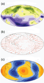
Figure 1: Geophysical phenomena coincident with circum-Pacific preferred longitudes of VGP paths: a) Non-dipole field anomalies, green inward flux and purple outward; b) Outermost core flow features with sites of convergence and divergence of longitudinal flows - the order of magnitude the flow velocity 10 km/a; c) Blue indicates fast P-wave velocities interpreted as anomalously cold lower mantle [7].

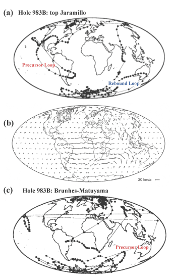
Figure 2: VGP reversal paths for the last two geomagnetic field reversals [7] and an outermost core flow model [13] a) N-R reversal at the top of the Jaramillo; b) Outermost core flow and; c) R-N reversal Brunhes-Matuyama.

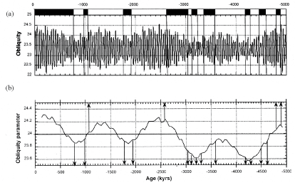
Figure 3: The occurrence of reversals for the past 5 Ma compared with a) The calculated obliquity, and; b) with a 5-point running average of obliquity maxima [18].

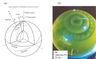
Figure 4: Precession and the geodynamo: a) The poles to the Ecliptic, the Core and Mantle rotation axes; b) Result of experimental run: note (1) The rotation axis for the core is displaced from the mantle axis, which is indicated by the point on the frame and (2) The band of small scale columnar rotations [22,23].

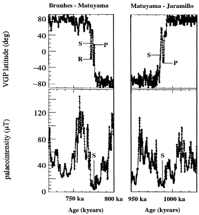
Figure 5: Ocean Drilling Project, Hole 983B: VGP latitude and paleointensity for Bruhnes-Matuyama (BM) and Matuyam-Jaramillo (MJ) reversals, S: Polarity switch midpoint minimum intensity; P: Precursor maximum; R: Rebound maximum [34].