
International Journal of Atomic and Nuclear Physics
(ISSN: 2631-5017)
Volume 6, Issue 1
Original Article
DOI: 10.35840/2631-5017/2524

Article Formats
Quantum Numerical Control of Nuclei†#
Table of Content
Figures
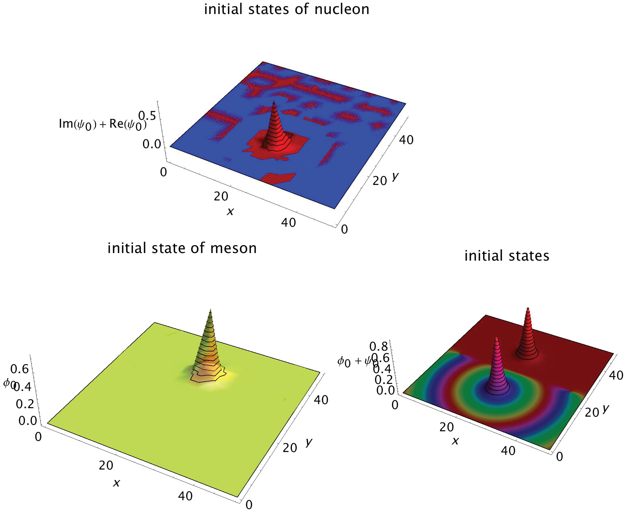
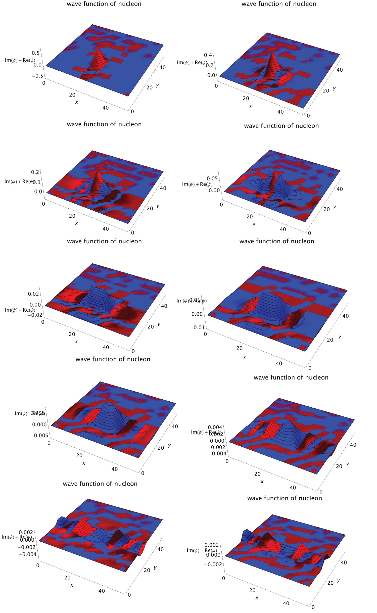
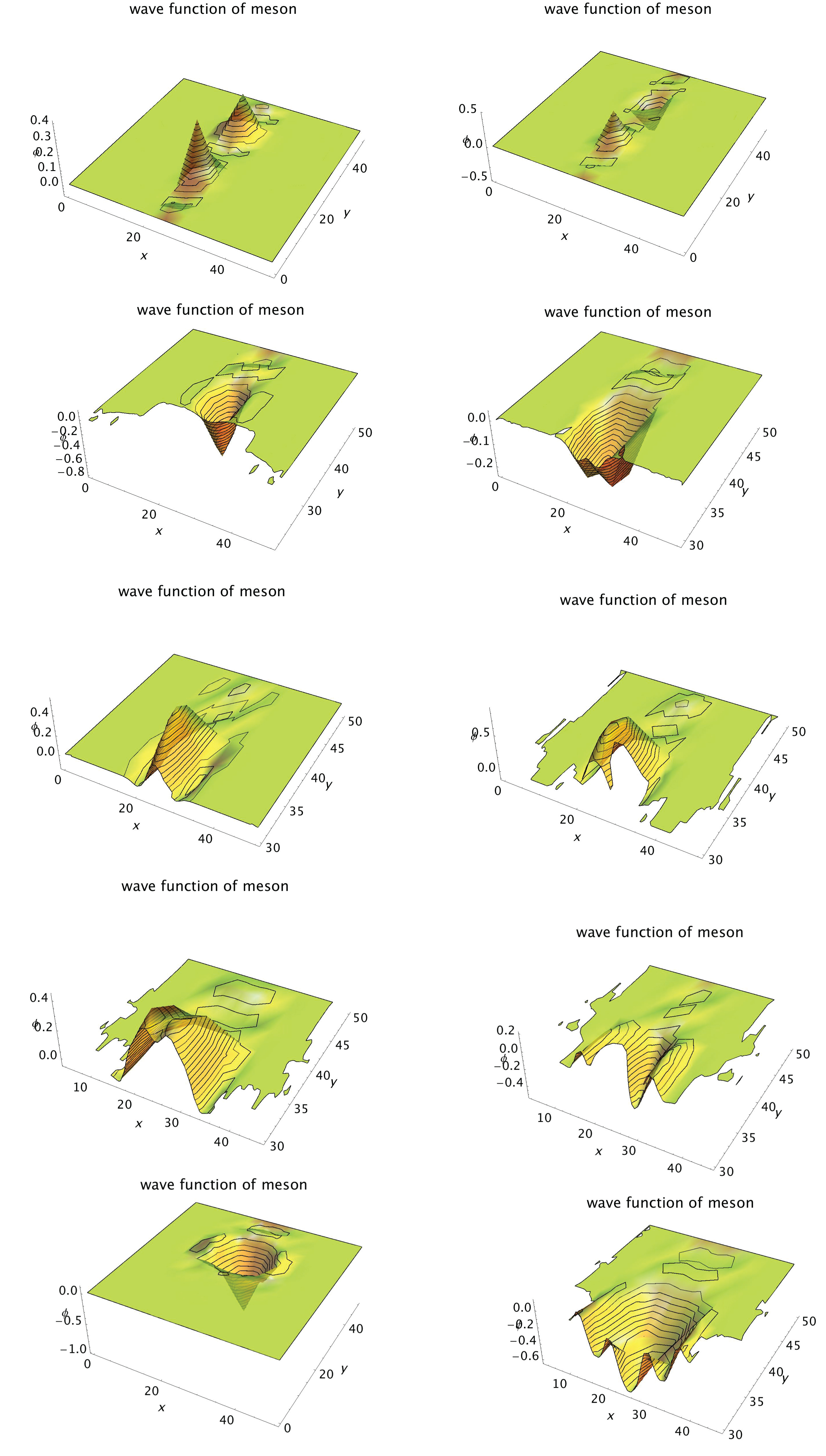
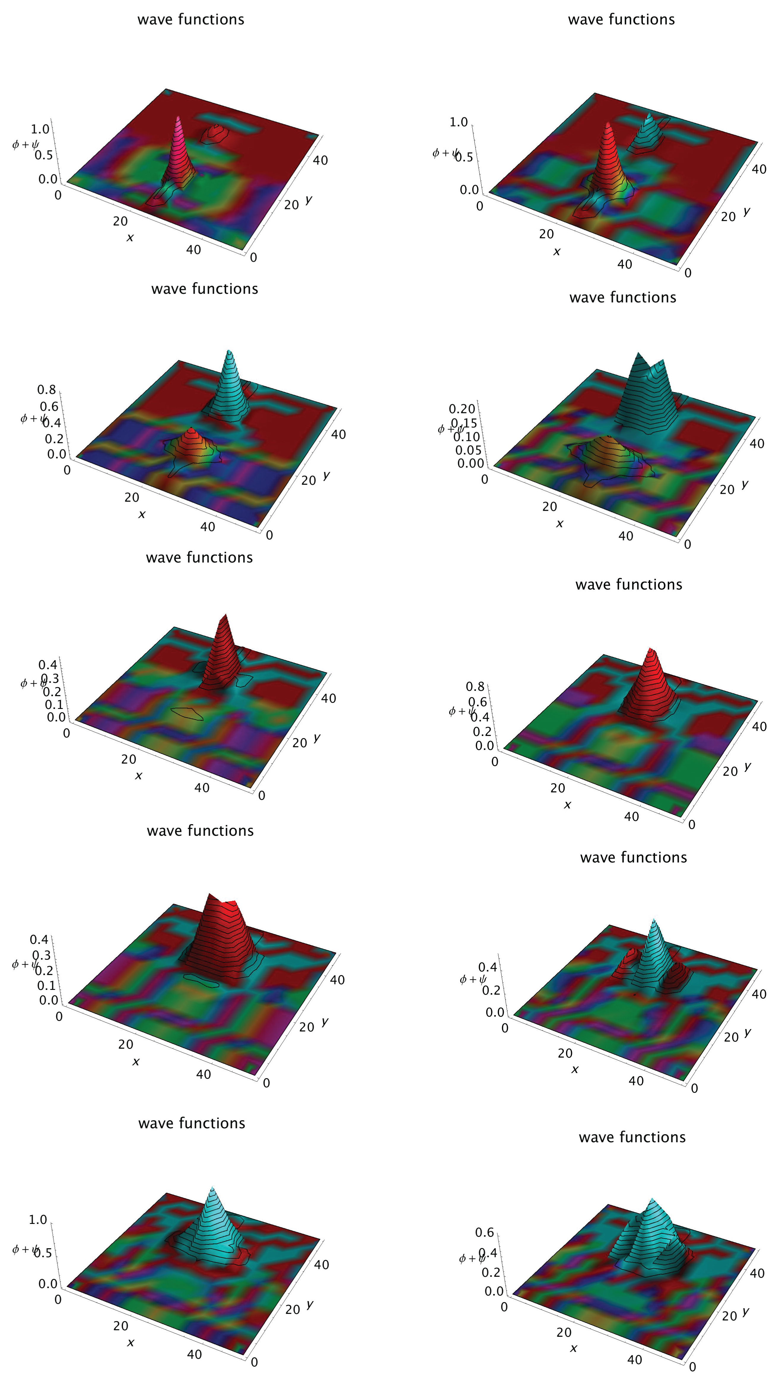
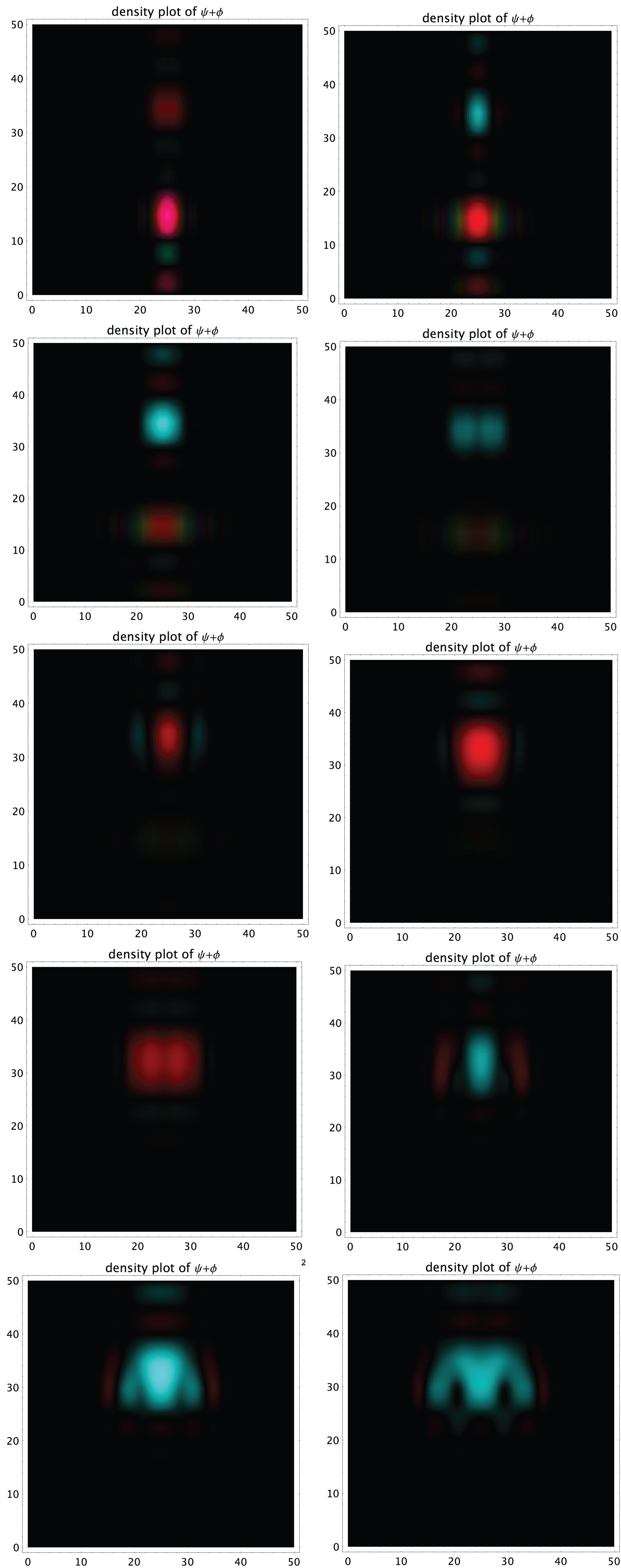
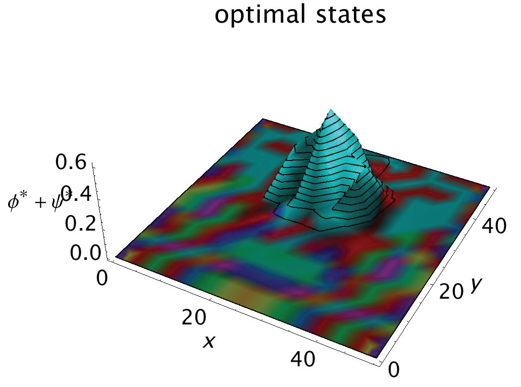
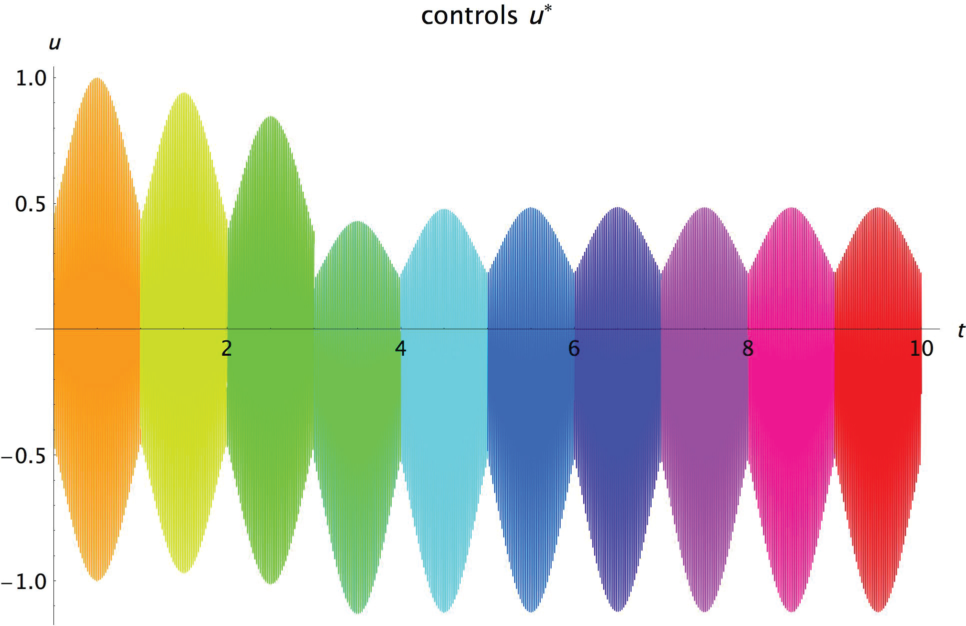
Figure 7: u*(t), n = 1, 2, ..., 10, before...
u*(t), n = 1, 2, ..., 10, before no interaction, after (n > 3) interaction happened.
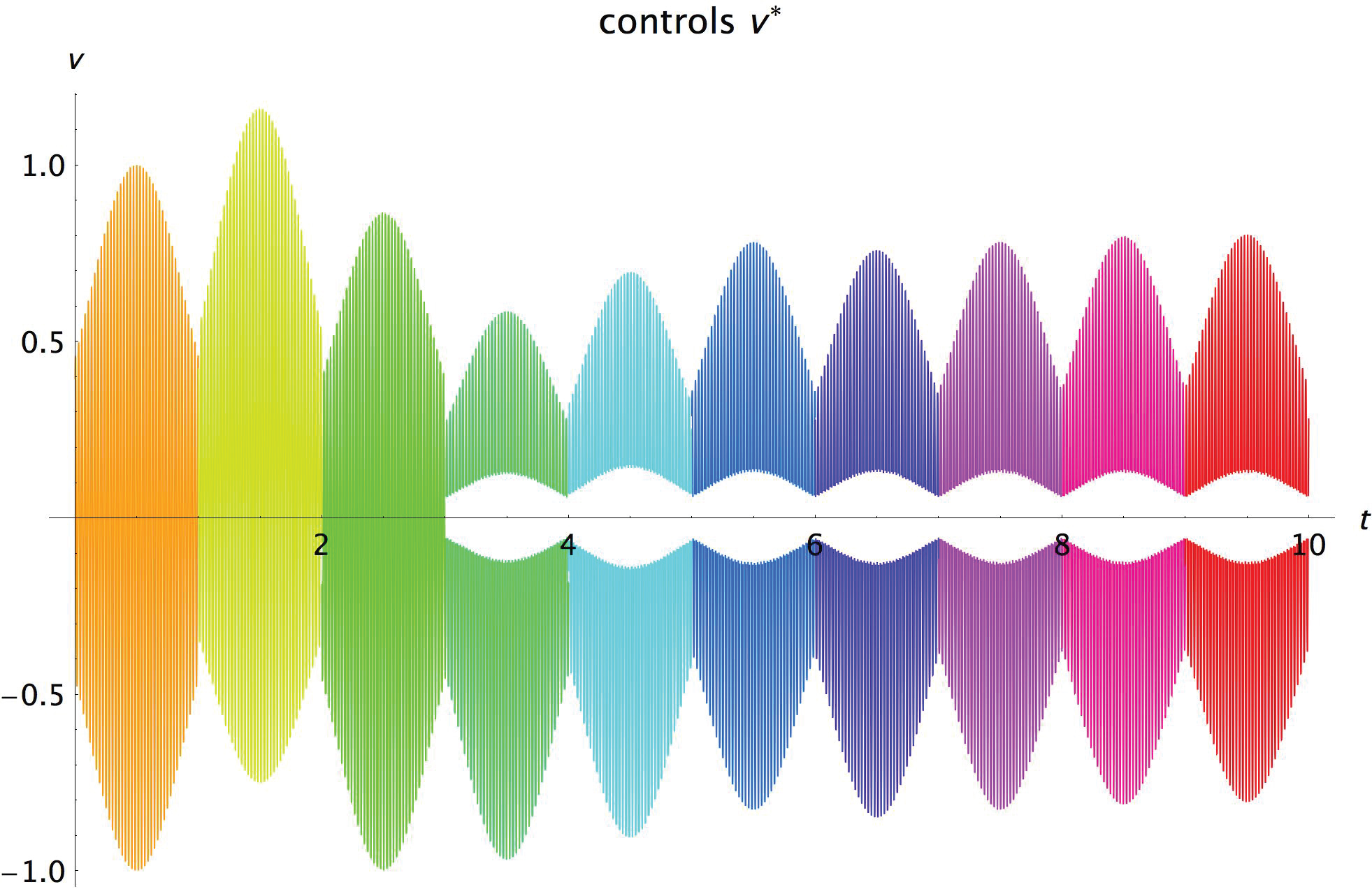
Figure 8: v*(t), n = 1, 2, ..., 10, before...
v*(t), n = 1, 2, ..., 10, before no absorption, after (n > 3) absorbed by nucleon, spatially surrounding nucleon.
References
- Berrios E, Gruebele M, Wolynes PG (2017) Chemical physics letters. 683: 216.
- Chu S (1991) Laser manipulation of atoms and particles. Science 253: 861.
- Chu S (2002) Cold atoms and quantum control. Nature 416: 206.
- Chu S (1998) Nobel Lecture: The manipulation of neutral particles. Review of Modern Physics 70: 685.
- Rabitz H, Regina VR, Motzkus M, Kompa K (2000) Whither the future of controlling quantum phenomena. American Association for the Advancement of Science 288: 824.
- Lasdon LS, Mitter SK, Warren AD (1967) The conjugate gradient method for optimal control problems. IEEE Trans, Autom Control 12: 132.
- Yukawa H (1934) On the interaction of elementary particles. I. Proceeding of Japan Physics and Mathematics Society 17: 48-56.
- Yukawa H (1937) On the interaction of elementary particle. II. Proceeding of Japan Physics and Mathematics Society 19: 14-23.
- Yukawa H (1938) On the interaction of elementary particle. III. Proceeding of Japan Physics and Mathematics Society 20: 24-45.
- Yukawa H (1938) On the interaction of elementary particle. IV. Proceeding of Japan Physics and Mathematics Society 20: 46-71.
- Wang QF (2006) Quantum optimal control of nonlinear dynamics systems described by Klein-Gordon-Schrödinger equations. Proceeding of American Control Conference 1032-1037.
- Wang QF, Rabitz HA (2007) Quantum optimal control of Klein-Gordon-Schrödinger dynamics in the presence of disturbances and uncertainties. Gordon Research Conference "Quantum Control of Light and Matter", Poster.
- Wang QF (2008) Theoretical issue of controlling nucleus in Klein-Gordon-Schrödinger dynamics and with perturbation in control field. Applied Mathematics and Computation 206: 276-289.
- Schrödinger E (1952) Dirac's new electrodynamics. Nature 169: 538-543.
- Lions JL (1971) Optimal control of systems governed by partial differential equations. Berlin, New York.
- Rice SA, Zhao M (2000) Optical control of molecular dynamics. John Wiley, New York.
- Schmidt B, Lorenz U (2017) Wavepacket: A Matlab package for numerical quantum dynamics. I: Closed quantum systems and discrete variable representations. Computer Physics Communications 213: 223-234.
- Schmidt B, Hartmann C (2018) Wavepacket: A MatLab package for numerical quantum dynamics. II: Open quantum system, optimal control, model reduction. Computer Physics Communications 228: 229-244.
- Adams RA (1975) Sobolev spaces. Academic Press, New York.
- Dautary R, Lions JL (1992) Mathematical analysis and numerical methods for science and technology. Berlin-Heidelberg-New York.
- Wang QF (2015) Identification problems of Klein-Gordon-Schrödinger quantum system control. Quantum Information Processing 14: 425-436.
- Wang QF (2018) Optimal control for Klein-Gordon-Schrödinger quantum system in complex Hilbert space. Proceedings of 37th Chinese Control Conference 8144-8149.
- Heisenberg W (1952) Production of mesons as a shock wave problem. Phys Bd 133: 65.
- Thaller B (2000) Visual Quantum Mechanics. Heidelberg-New York.
Author Details
Quan-Fang Wang*
Mechanical and Automation Engineering (Former), The Chinese University of Hong Kong, Hong Kong
Corresponding author
Quan-Fang Wang, (Former) Mechanical and Automation Engineering, The Chinese University of Hong Kong, Shatin, N.T., Hong Kong.
Accepted: March 02, 2021 | Published Online: March 04, 2021
Citation: Wang QF (2021) Quantum Numerical Control of Nuclei†#. Int J At Nucl Phys 6:024.
Copyright: © 2021 Wang QF. This is an open-access article distributed under the terms of the Creative Commons Attribution License, which permits unrestricted use, distribution, and reproduction in any medium, provided the original author and source are credited.
Abstract
Quantum control of elementary particle at nucleon had already been investigated for a couple of decades at the frontier area both in quantum physics and system control. At the nucleus, a kind of control for particles motion had been considered in the form of Klein-Gordon-Schrödinger equation, which is a system describing the Yukawa interaction between nucleon (e.g. proton, neutron) and meson. The aim of this paper is trying to find an external force to act at one of the particles to change the particle from its ground state to reach its exciting state. A lot of very interesting results had been obtained and make a clear picture with numerical approximate and computational approach. For interpreting, the meson can escape from the cloud of proton 'p' to join the neutron 'n', it turned the proton 'p' to a new neutron, and neutron 'n' to a new proton. The Yukawa interaction can be incident naturally, whether it can be controlled? The control either be accelerated or slow-down the speed of meson exchange effect. Corresponding to theoretical results, two dimension control of heavy particles had been utilized in experimental aspect, it needs to seek control input to make it happened. For instance, using shaped laser pulse, particles beam, etc. Taking this opportunity, it is delighted to report the detailed conclusion of nuclei control issues and explore future research direction.
Keywords
Quantum control, Klein-Gordon-Schrödinger equation, Nucleus, Numerical approach
Introduction
In the physics, chemistry and mathematics fields, quantum control had been considered in literatures and contributed papers world widely. By the investigation of existing research works, it is easily find for us that the recent development and progress in the quickly growing areas. In fact, there are various breakthroughs had been made for control of particles at the quantum physics subject. In the frontier realms, one can list the most highlighted milestone works such as trapped cooling atom with laser technology see [1-4] controlling molecules rearrangement and dissociation see [5] controlling molecules within chemistry reaction (e.g. break the weak bond); Iteration learning controlling (e.g. finding optimal set instead of one particular shaped laser wave functions [6]), so forth. It is also extended to control of motions of atoms and molecules; Control of their structures; Control quantum qubit NOT gate; Control of logic quantum qubit computations. With these amounts of outstanding research achievements (cf. [7-10]), a great deal results had already been obtained in the past several decades (cf. [11-13]). Certainly, it would be a convinced standpoint to boost the field to the future.
Eventually, at the view of physics, it extremely needs to solve the problems which still exist in the majority number. Control of nucleus had been considered for a long time in a variety methodologies at the real laboratory, It is apparently could not be directly realized at present experimental equipment's. However, theoretical control nuclei could be predictively worked at the academic level. It keens to have continuously and mutated study to seek a pathway or shortcut to control elementary particles anticipatively. A physical model of control theory of quantum system and computational simulation of numerical experiments would be taken account into this work.
Couple Heavy Particles
Firstly, let us introduce Klein-Gordon-Schrödinger (KGS) equation in the nucleus with real atomic units. Suppose Ω is an open bounded set of spatial space R3 and set Q = (0, T ) × Ω for time T > 0. The i denote the unit of imaginary part of complex space. For the description of nucleon particle has the form of Schrödinger equation (cf. [14])
Where ψ denote complex-valued function representing probability density of nucleon field with initial ground state is reduced Planck constant, M is the mass of nucleon, and e is the charge of proton. The simultaneous equation of (1) is the Klein- Gordon dynamics, which described the motion of meson by
Where denote real-valued function representing probability density of meson field with initial ground states given by and . c is speed of light. m is mass of meson, is charge of meson. Definitely, the physics model consists of (1) and (2) represents the motions of two heavy particles in the presence of Yukawa interaction see [7-10]. Two functions u and v represent control inputs corresponding to external forces such as ultrashort (e.g. femtosecond/attosecond) infrared laser pulse (e.g. terahertz) in real laboratory experiments as in [15,16]. The shaped laser pulse might be suitable to be manipulated for the purpose (cf. [17,18]).
Quantum Control of Nuclei
Let be a closed and convex admissible set of . Without lost of generality, control variables usually taken as time depended only functions, denote as u(t) = (u(t), v(t)) for simplification, its belonging space denoted as = L2(0, T )2. Introduce two Hilbert spaces with usual norm and inner products (cf. [15,19]). Hence, two embeddings in Gelfand triple space V ↪ H ↪ V' are continuous, dense and compact, where i.e. is conjugate space of V (cf. [15,20]). For meeting the realistic simulation, taking both real spaces for real part and imaginary part of wave function , and taking real space for wave function as usual in here. For complex valued function , if necessary, consider real part only for simplifying. Denote for wave function.
Definition 1: If functions belong to the space defined by
It is solution space. If then inner product is defined by
Then, inner product induced norm of solution space defined by
Hence, become a Hilbert space equipped with above inner product and norm.
Definition 2: Let T > 0, the pairing ( , ) are weak solutions of (1) and (2), if , ,
and satisfy
for all and such that .
The cost function associated with KGS states system (1)-(2) is taken as
for all where are target exciting states, and are final observed quantum states, respectively. Here, and are penalty weighted coefficients for balancing the evaluates of system and running criterias.
As is well known, quantum optimal control is to solve two fundamental problems:
i). Find an element u* = (u*, v*) such that
ii). Characterization of u*.
Such u* is called quantum optimal control for Klein-Gordon-Schrödinger system (1)-(2) subject to cost function (4).
Theorem 3: For given , if is convex and closed (bounded) subset of , then there exist a unique weak solution of KGS system (1)-(2) at space , and has inclusive .
Indeed, using Faedo-Galerkin method and citing [21,22], a prior estimates for and can be obtained by routing manner at solution space.
For via the virtual of Theorem 3, there exists a unique weak solution of KGS system (1)-(2) in the solution space W (0,T;V,V). Hence there is a solution mapping from control space to solution space : → W (0,T;V,V), which is continuous mapping. In here, is called the states of KGS control system (1)-(2).
Theorem 4: Given , if space is bounded closed convex space, then there is at least one quantum optimal control of Klein-Gordon Schrödinger system (1)-(2) subject to cost function (4).
Follow article [22], straightforwardly to get the proof of Theorem 2 at real spaces.
Theorem 5: Given and . For be a bounded closed convex space, then quantum optimal control u* = (u*, v*) for cost function (4) subject to states system (1)-(2) is characterized by simultaneously optimality (Euler-Lagrange) system:
Where are weak solutions of adjoint systems (6) corresponding to solutions in states system (5) respectively. Clearly, inequality (7) is well known as the necessary optimality condition.
Using the definitions of weak solution and weak form (3) in the defined solution space , one can quickly get full proof as analogical manipulation citing [11,13,21,22].
Numerical Approach
A lot of successful algorithms for finding optimal control of quantum system, for example, there are iteration learning algorithm; Genetic algorithm; evolutional algorithm, etc. To calculate quantum optimal pairing u* and v*, in this paper, is for seeking quantum optimal u*, a reasonable semi-discrete algorithm (spatial variable x discrete, time t continuous) is employed for control in nucleus. In there, the finite element method is used in computational approach in the form of variational method at Hilbert spaces. Quadratic base function is adopted in finite element approximate. Further, a modified nonlinear conjugated gradient method (CGM) is utilized in the system optimality minimization. Particularly, the wave-particles duality and uncertainty principle of Heisenberg [23] allow the ideal and reliable scheme. The convergence order is guaranteed (cf. [6]) for first order O(h). Roughly introduce the structure of numerical algorithm. Let 0 = t0 < t0 < • • • < tN < tN+1 = T be a partition of the interval [0, T] into subintervals Ie = [te-1, te) of length dte = te - te-1, e = 1, 2, • • • , N + 1. The corresponding spatial interval would be Je = [xe-1, xe] of length e = 1, 2, • • • , N + 1. Let Vh be a approximate space expanded by quadratic basis functions (i = 1, 2, 3, e = 1, 2,..., N + 1), which continuous on each interval Je given by
Using to construct the total approximate solution for j-th nucleon and meson as
Where , are indeterminate coefficients, which will be solved by fourth order Runge-Kutta method as in [11]. Assume that is valid at one iteration step, its corresponding approximate solutions are and . Denote are the total number of involved nucleon and meson, respectively. Consider minimization problem for discrete objective functions:
A modified nonlinear conjugate gradient method (CGM) is used for minimization problem in (8). The detail computing procedure can be find in [11] for one dimension.
Theorem 6: For finite element problems (8), there exists at least a minimizer of sequence .
Theorem 7: For minimizing the control sequence , extract a subsequence, again denoted by which convergent to in , to minimize the discrete problem (8).
By extended to two dimension case, the convergence of iteration procedure in minimizing Jh is guaranteed in [6], and the approximate control converges to in the order of O(h) as h → 0.
Demonstration Results
Set physics constant = M = m = c = 1, e = = 1. Nucleon and meson particles motions are considered in two dimensional spatial space [0, X] × [0, Y], where X = 50(μm) and Y = 50(μm). Take t0 = 0.0(fs), T = 20.0(fs) and time interval ∆t = 1.0(fs). Assume the stop criteria ε = 10-35 in minimization scheme. Denote center coordinate x0 of domain. Define two appendix functions for initial states configuration:
Where, v1 and v2 are velocities of nucleon and meson, respectively.
Use Mathematica for three sets of simulation experiments.
Ex. a) Two particles simulation
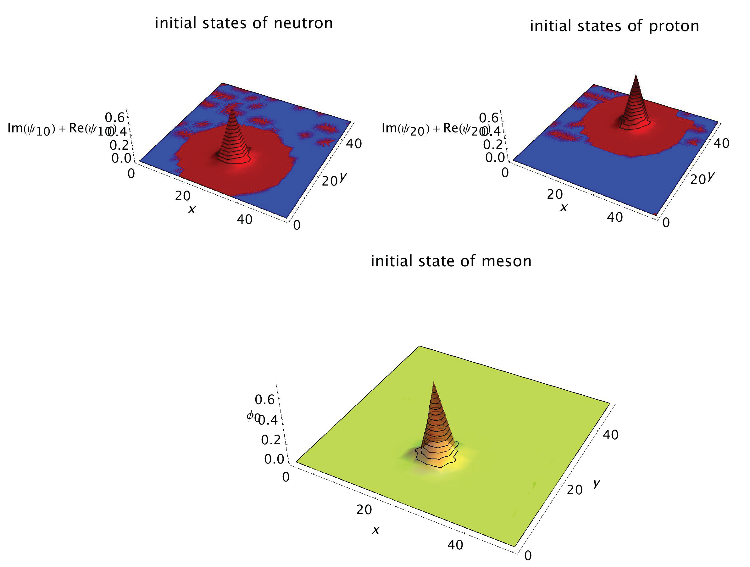
Set x coordinate location center x0 = 25.0(μm), two particles locations at y coordinate are y10 = 15.0(μm) and y20 = 35.0(μm). Precisely, nucleon located at (25,15) and meson located at (25,35) in the (x,y) plane. In physics, it will be n + π+ → p, one proton will be gotten. Their wave propagation velocities v1 = 5/12 and v2 = -5/12. Therefore, initial ground states can be given by
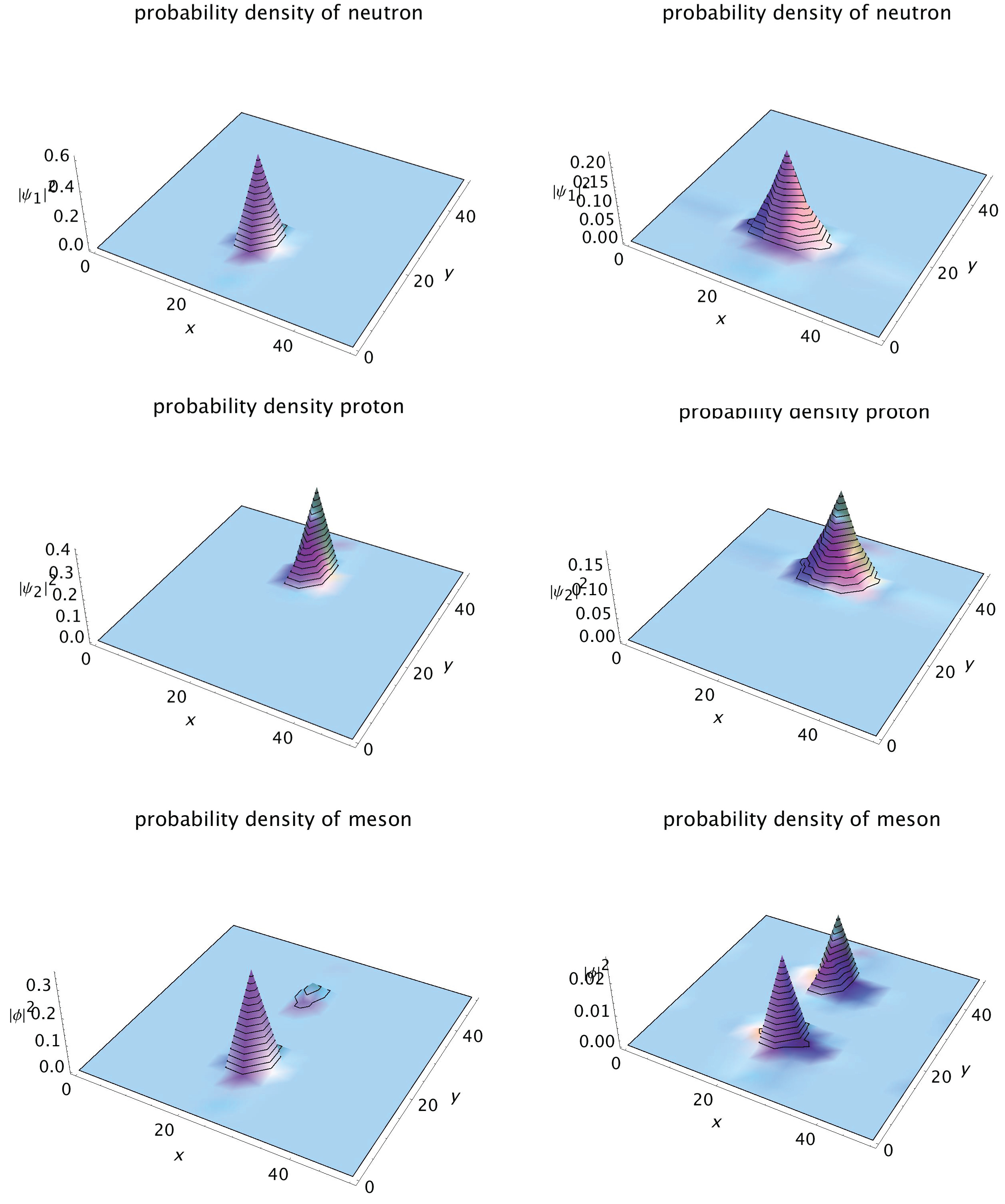
The graphics of and are plotted in Figure 1, respectively.
Take target quantum excited states
Assume the iteration step nn, and define Gaussian enveloped function Set initial control input for nucleon and for meson. Notice that the last iteration wave function is not used in next step control: . It means that quantum dot at spatial location is not depended on time. Wave function has the same fashion at each iteration. Figure 2 given the states transform of nucleon.
Figure 3 given the states transform of meson.
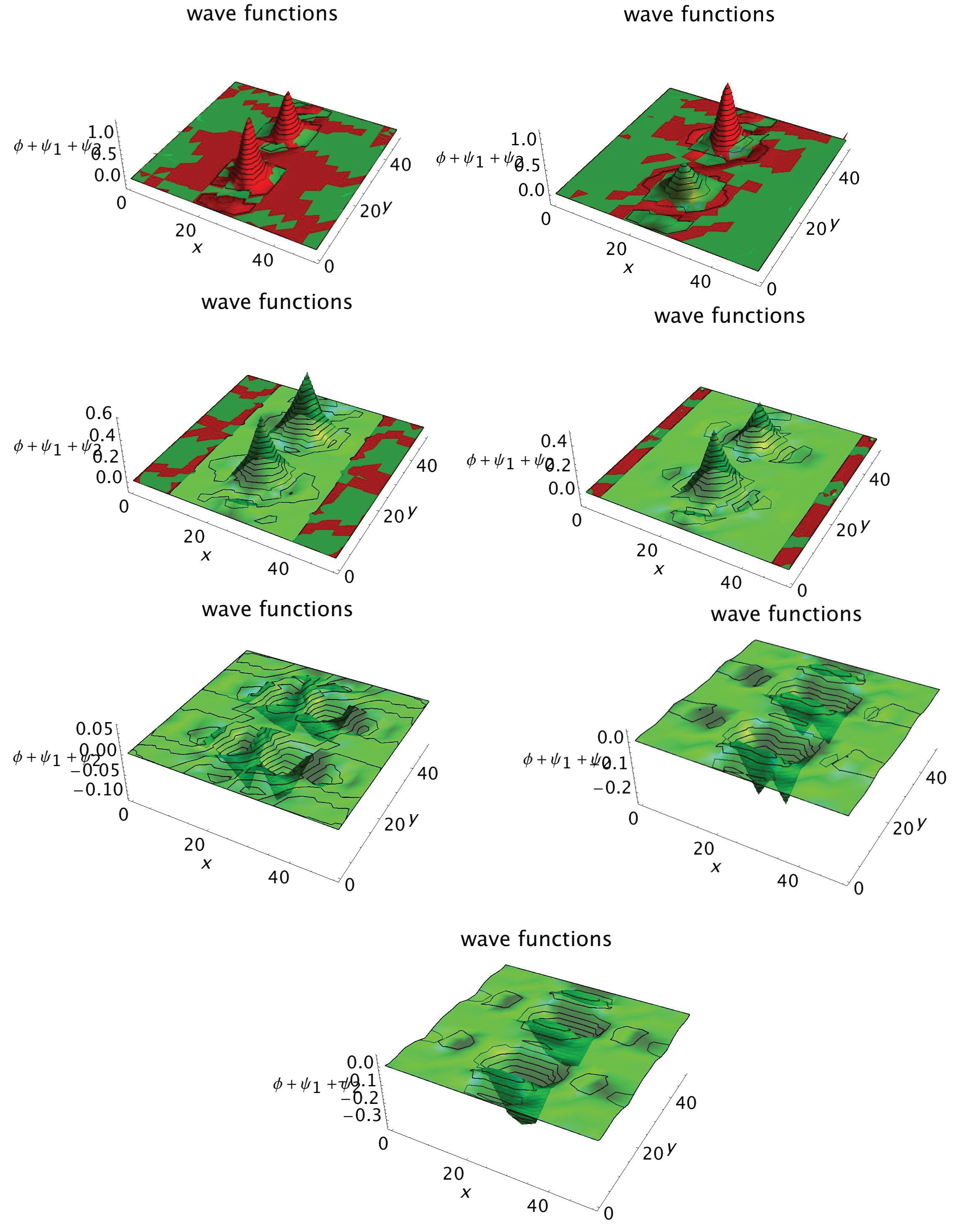
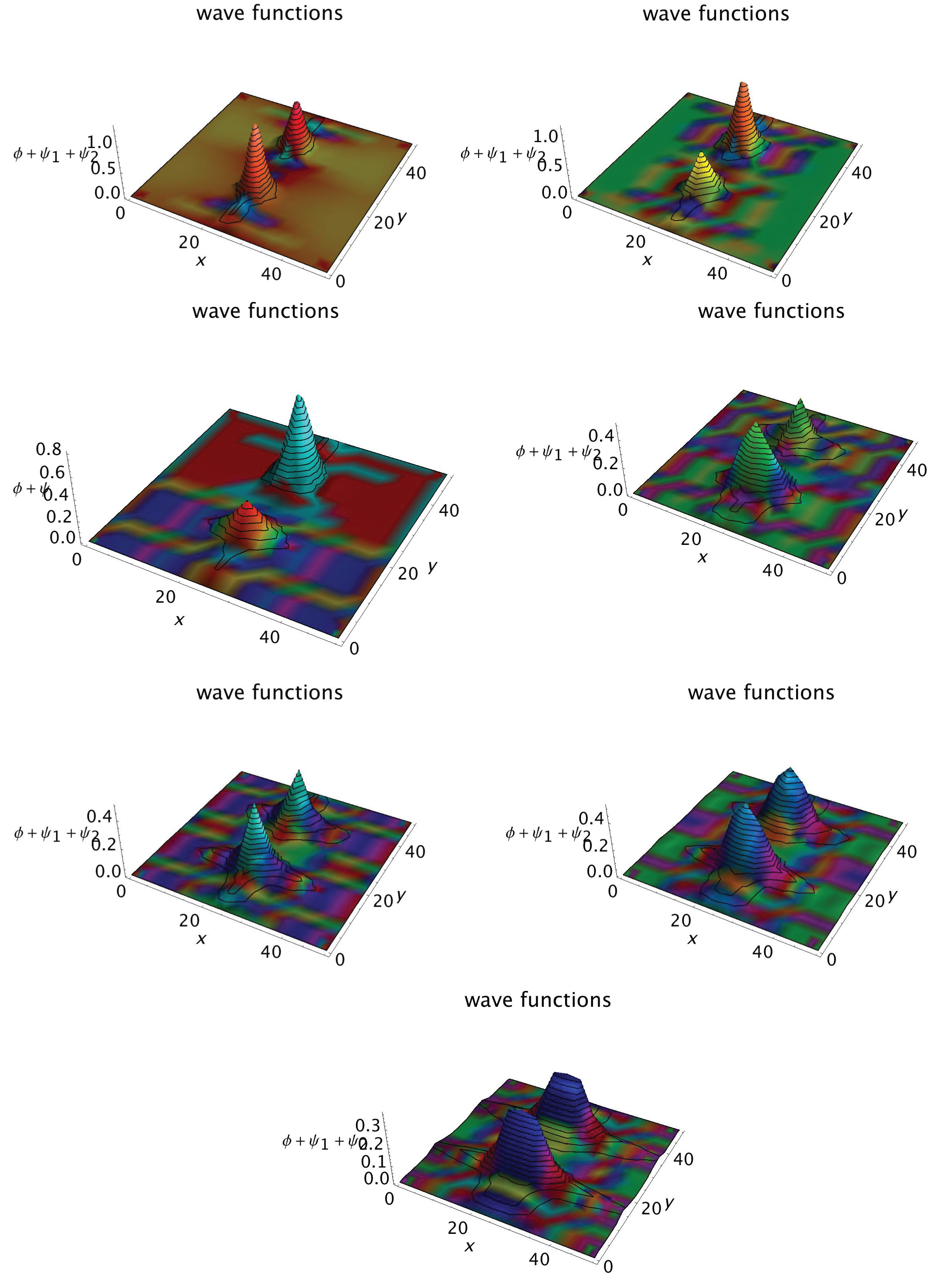
Figure 4 use Mathematica VQM package1, [24] 3D plot of wave function .
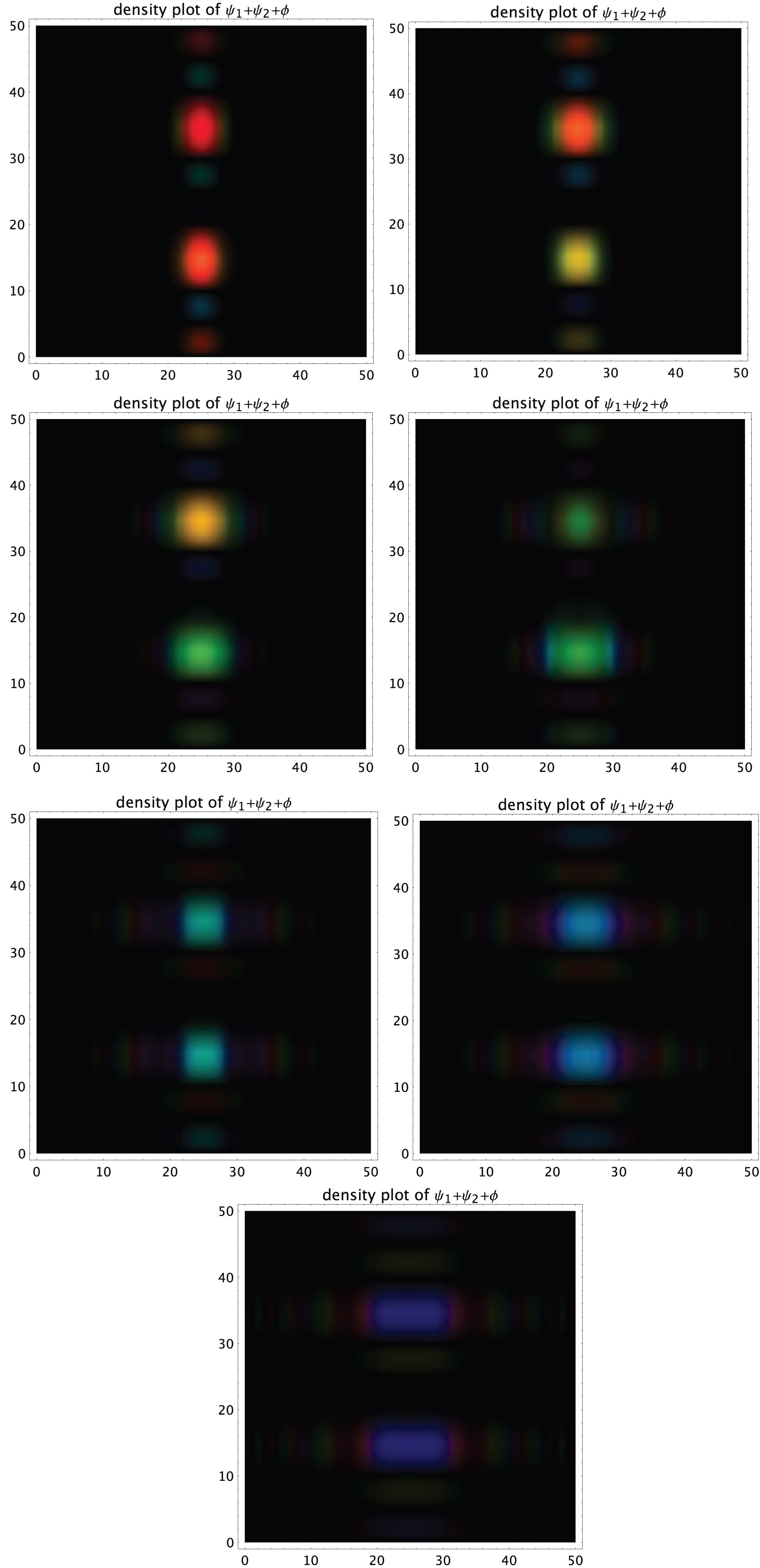
Figure 5 is the probability density plot of .
At Figure 4 and Figure 5, control function u and v act at the nucleon and meson, and force particles reach optimal states at final step. They replaced their spatial position and changed the representing color. It means that neutron absorb meson become proton (e.g. n + π+ → p), similarly simulation can be obtained for proton emit meson become neutron (e.g. p + π- → n). Observe imaginary part coefficients of used control function at each iteration, the gauge is agree with realistic atom unit. Figure 6 is the optimal state of .
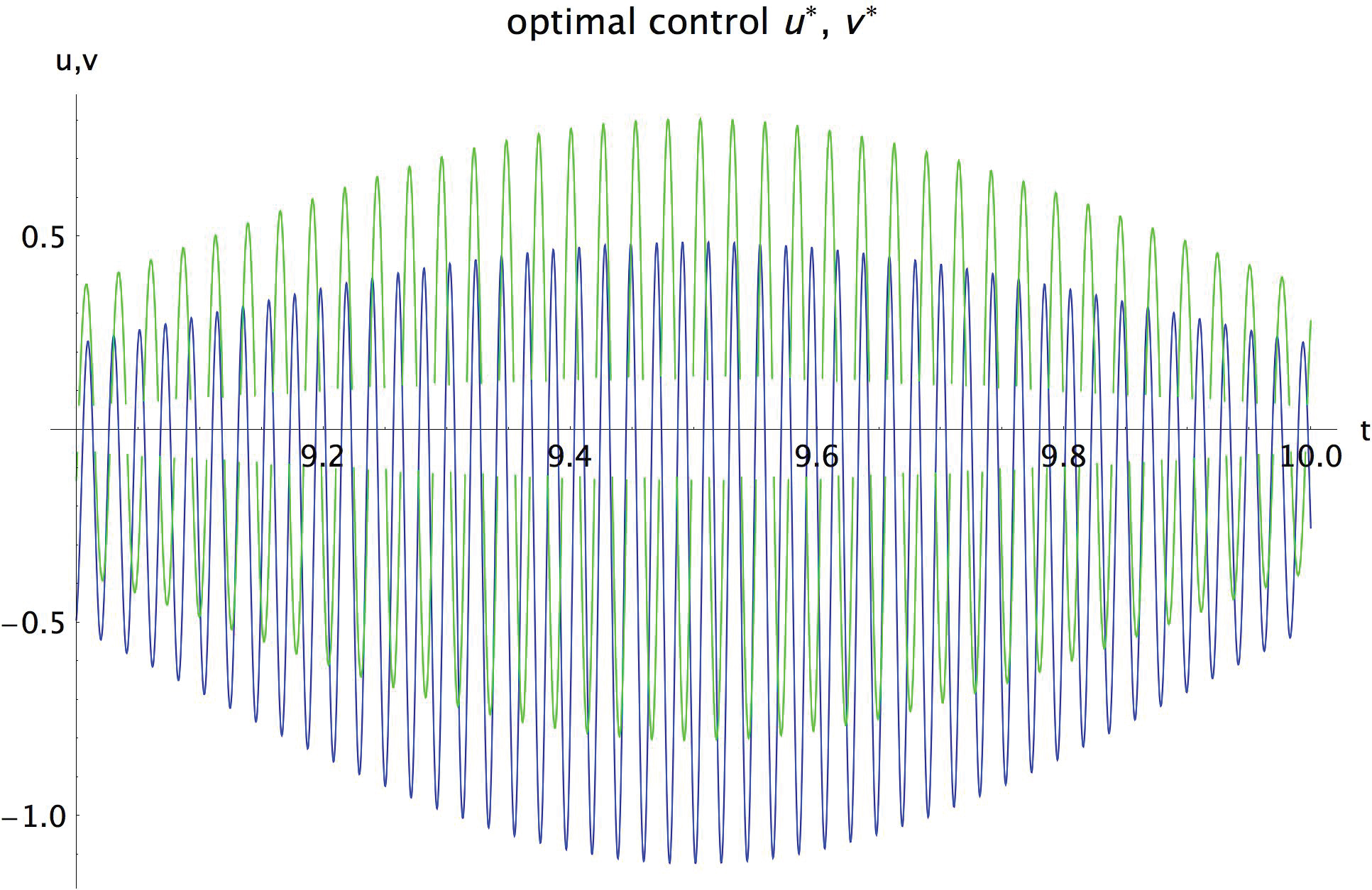
The graphics of u*(t) and v*(t) at all iterations are plotted in Figure 7 and Figure 8.
Notable, there is a gap in the plot of v* at Figure 8. Before the gap, meson is out of the nucleon cloud, after the Yukawa interaction, meson motion moved into (absorbed by) the cloud of one nucleon, but they had neither been completely reached the nucleon core itself, therefore, the probability distribution of meson will be likely surrounding the nucleon, and its (external) control input cannot be acted at this area. In the spatial dimension, the empty gap definitely appeared. Statistically, that is to say, it cannot find the meson at gap space. As is known that the radius of neutron is rn = 1.11492 × 10⁻¹³ m, the radius of proton is rp = 1.113386 × 10⁻¹⁵ m, the radius of pion meson is rπ = 1.53472 × 10⁻¹⁸ m, and the electron radius is re = 2.817939 × 10⁻¹⁵ m. The guess amplitude of the gap is small than the radius of nucleon. Very interesting, in Figure 7 they are no gap at nucleon control function at all, owing to its control input can be acted at the nucleon itself either not absorbed (no emission) or absorbed (emission) meson. Both in Figure 7 and Figure 8, the amplitudes are clearly changed after n = 3, it reflects that the positions of nucleon and meson are slightly changed.
Using quark calculation to know that neutron n = udd (spin 1/2, charge 0), proton p = uud (spin 1/2, charge +1), in here up quark , down quark , and meson pion (no spin, charge +1), where anti-quark . Then to have . In resultant, there is one quark u and one quark d not changed, they combine a new quark u of to compose proton, meanwhile, destroy (annihilation) a quark d and anti-quark . The mass of up quark is 5MeV/c2, and the mass of down quark is 10MeV/c2, where 1MeV/c2 =1.782677 × 10⁻³⁰ kg. It means that d is bigger than u, then neutron n = udd is bigger than proton p = uud. In scientific calculating, the mass of neutron n is 939.6MeV/c2, and proton p is 938.3MeV/c2. Symbolically, 2 big quantum dots and 1 small quantum dot 2 small quantum dots and 1 big quantum dot. Confidently, it is accordance with the real physical facts.
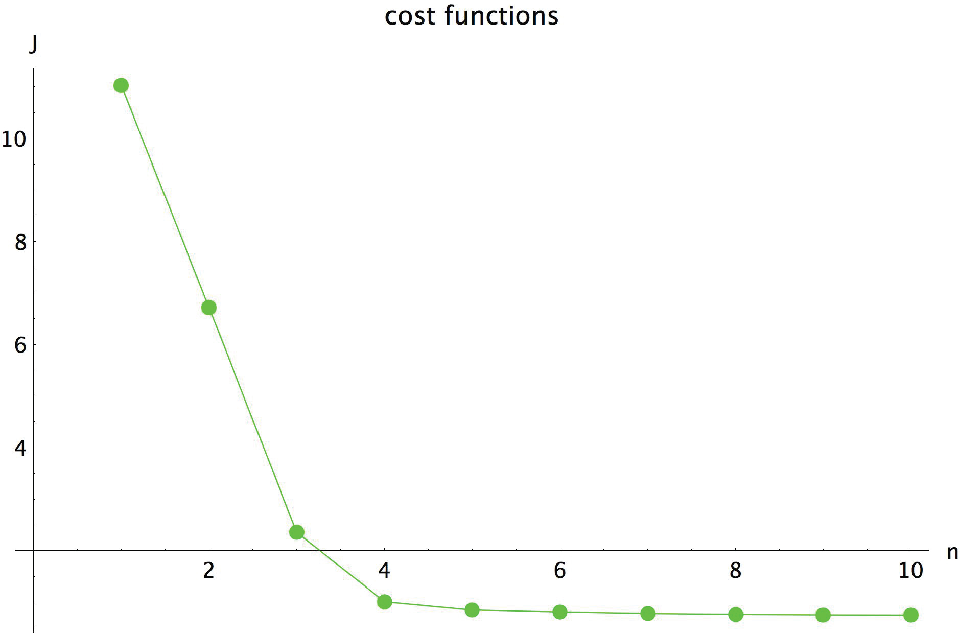
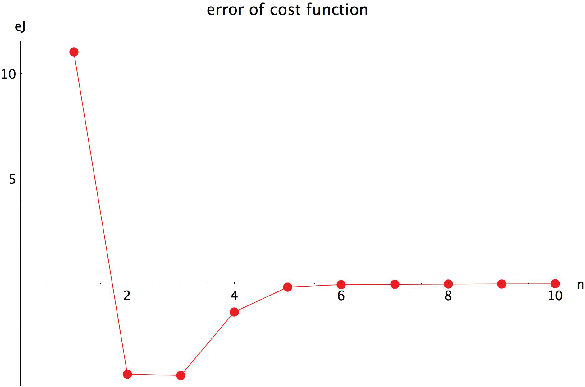
The optimal cost function value J(u*) = 0.747069, and minimization error eJ(u*) = 0.00563018. Quantum optimal control is calculated,
Figure 9 is for their graphics.
The cost values J(u) and error values eJ(u) are shown in Figure 10 and Figure 11, respectively.
Non-control. For the comprising, non-control iteration data had also been obtained, and their values are shown in Table 1. Clearly, control is accelerating the meson exchange effect in the Yukawa interaction. The energy is not conserved at whole control process. The value of cost function, and its error at each iteration step, see Table 1.
The implementation is taken place at the device with CPU 1.3GHZ, MacOS GPU v3. Total computing time is 2950.12 second. The used maximum memory is 2262.107390 bytes.
Ex. b) Three particles simulation
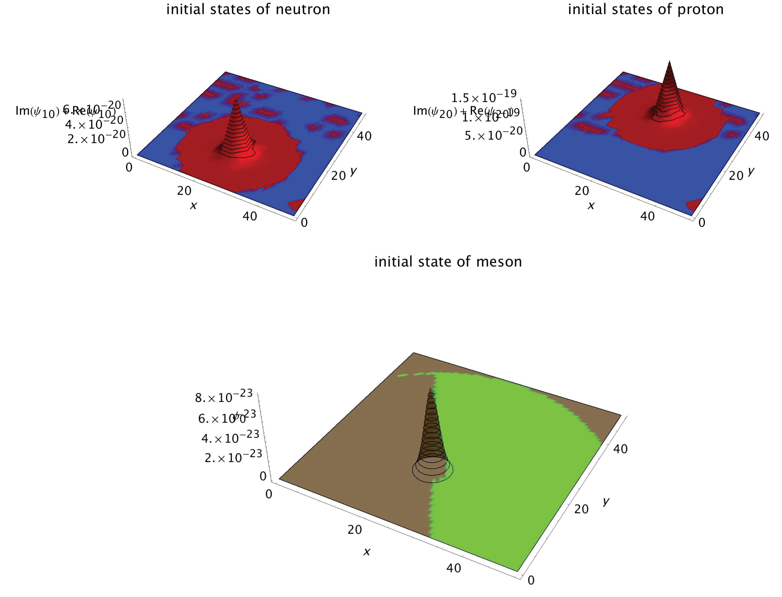
Set proton (neutron and meson) located at (25,15) and neutron located at (25,35) in the (x, y) plane. Meson wave propagation velocities v1 = 5/12 or v2 = -5/12 between proton and neutron. Set initial control inputs for proton, no control for neutron, and for meson. Therefore, initial ground states can be given by
The graphics of , and are plotted in Figure 12, respectively.
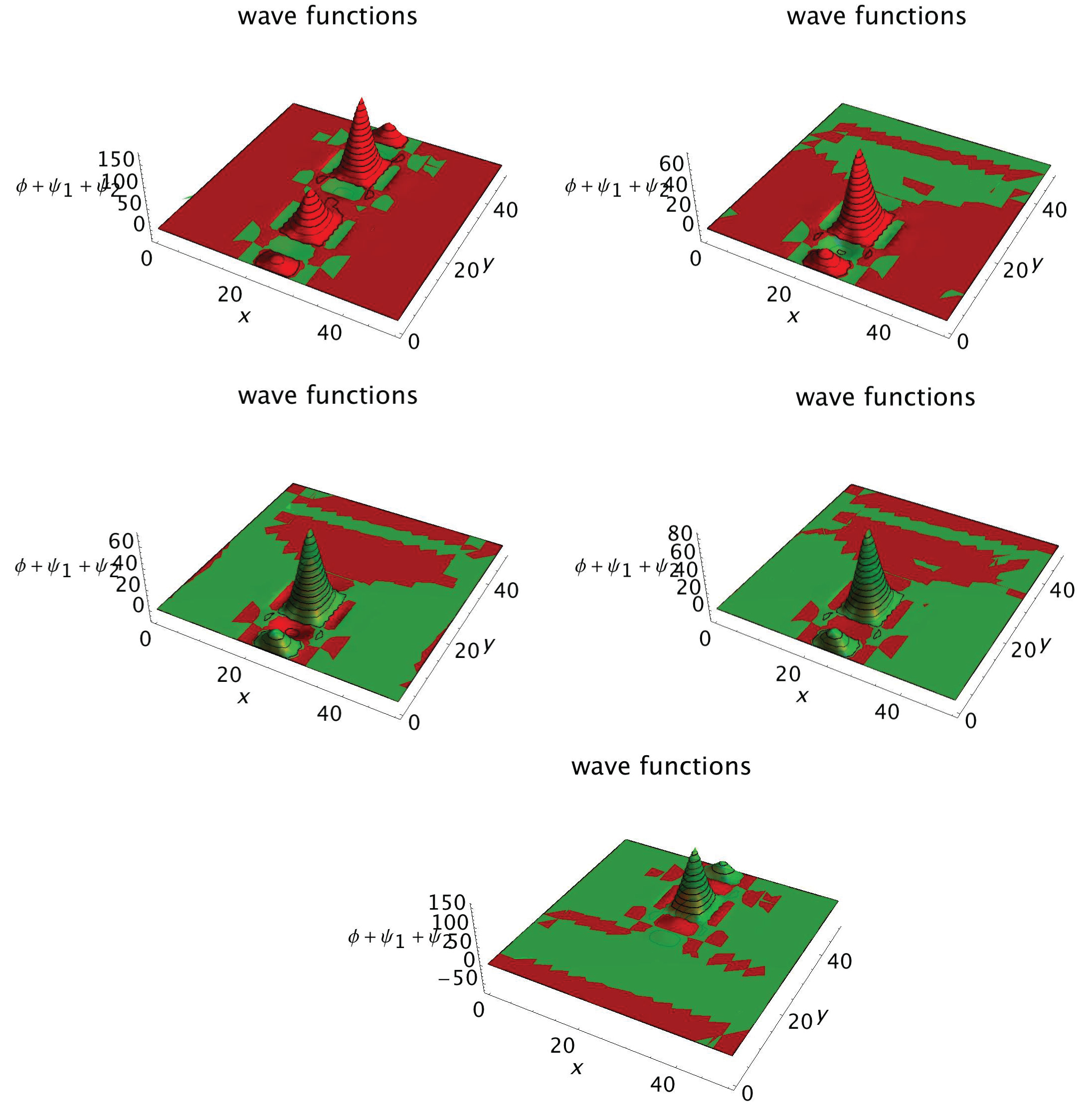
Notice that neutron and meson is located at same position. It means that proton is located at (25,15) initially. Physically, it will be n + π+ → p and p, two protons will be gotten. Figure 13 is their 3D plot of wave functions at each control iteration.
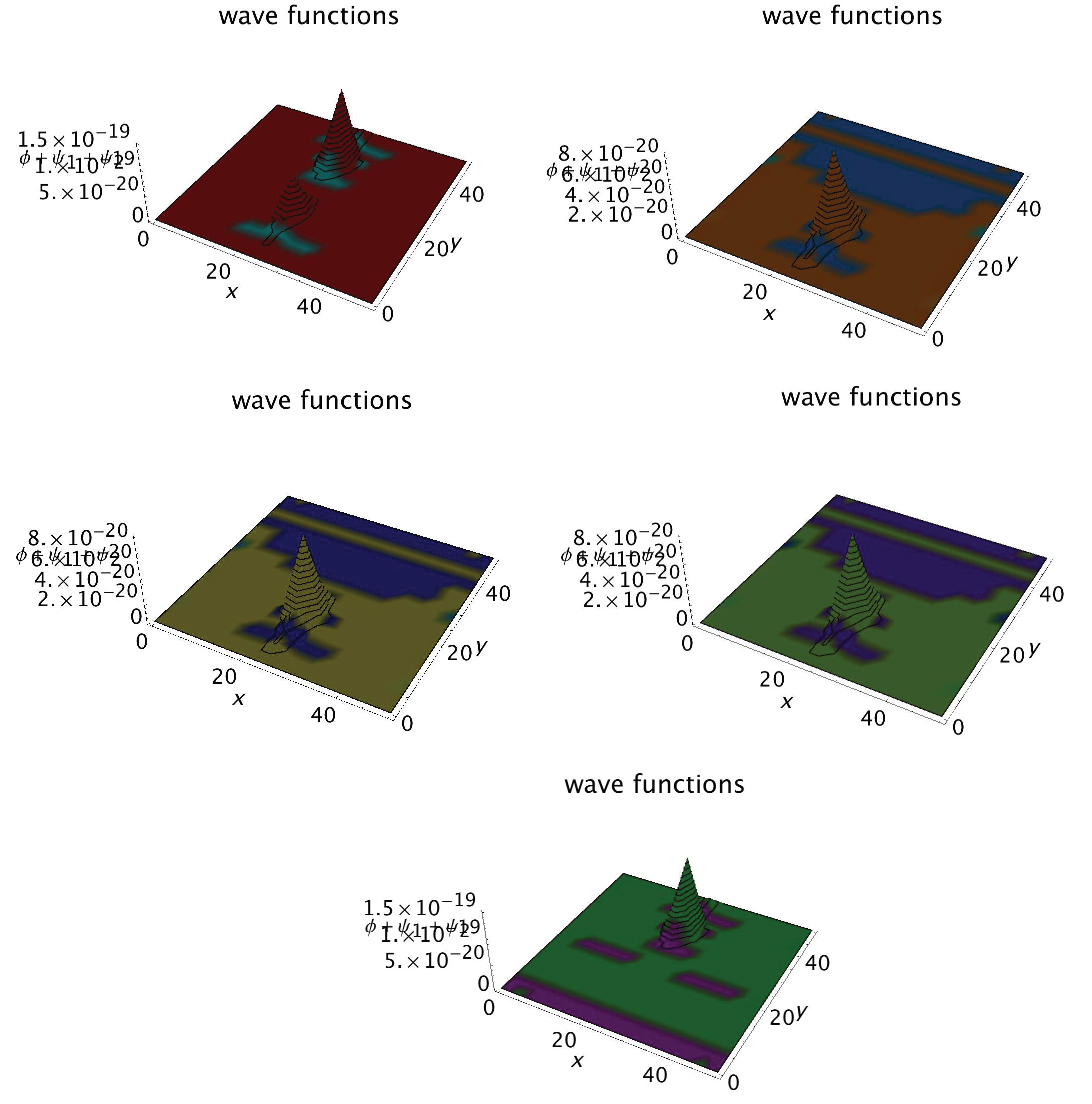
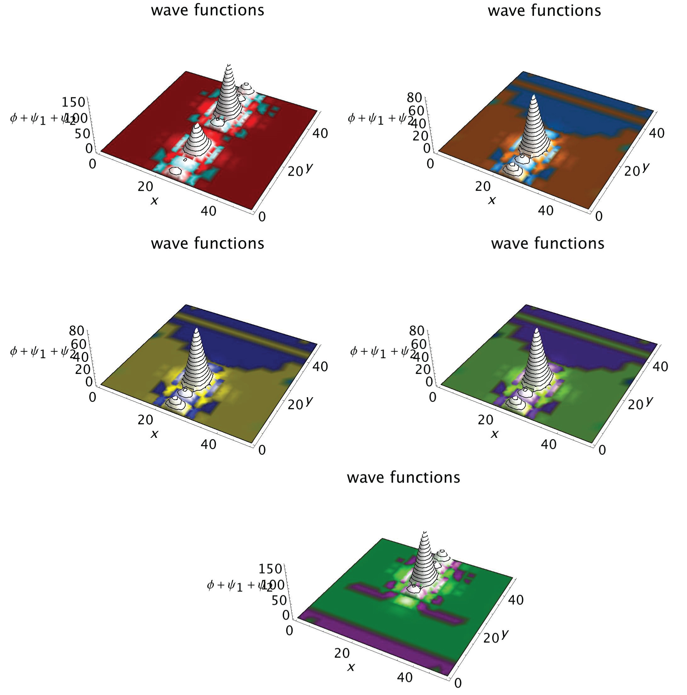
More precisely status, use Mathematica VQM package to execute 3D plot of wave functions at each control iteration Figure 14.
Figure 15 is the probability density plot of .
Wigner function for representing probability density and are compared here Figure 16.
Ex. c) Three particles with real atomic unit and physics constants
Take proton mass Mp = 1.67262 × 10⁻²⁹ g, neutron mass Mn = 1.67493 × 10⁻²⁹ g, and meson mass Mm = 2.305589 × 10⁻³⁰. The speed of light c = 2.99792 × 10⁸, the reduced Planck constant = 1.0545715964207855 × 10⁻³⁴, electron charge e = 1.602176462 × 10⁻¹⁹. Particles located at the same position as Ex. b). In physics, meson speed vm = 0.998c between proton and neutron. It will be n → π-1 + p and p, meson will be appeared with neutron and proton, respectively. Notice that the domain of spatial variable is taken as Ex. b) for the visualization, and set meson wave propagation velocities v1 = 5/12, v2 = -5/12 for continuity of algorithm. For much more delicate physical control issues using this paradigm, it concerns future work beyond this section. Fortunately, current simulation is the foundation of realistic physical control of KGS system. Ex. c) will suggest that control can be actually executed at the physics field. Certainly, further demonstration in the viewpoint of physics area will appear sooner after. Set initial control inputs for neutron and proton, and for meson. Therefore, initial ground states can be given and expressed by
The graphics of and are plotted in Figure 17, respectively.
Figure 18 is normalized 3D plot of wave function at each control iteration.
Precisely, Mathematica VQM package to do 3D plot of wave functions at each control iteration as Figure 19.
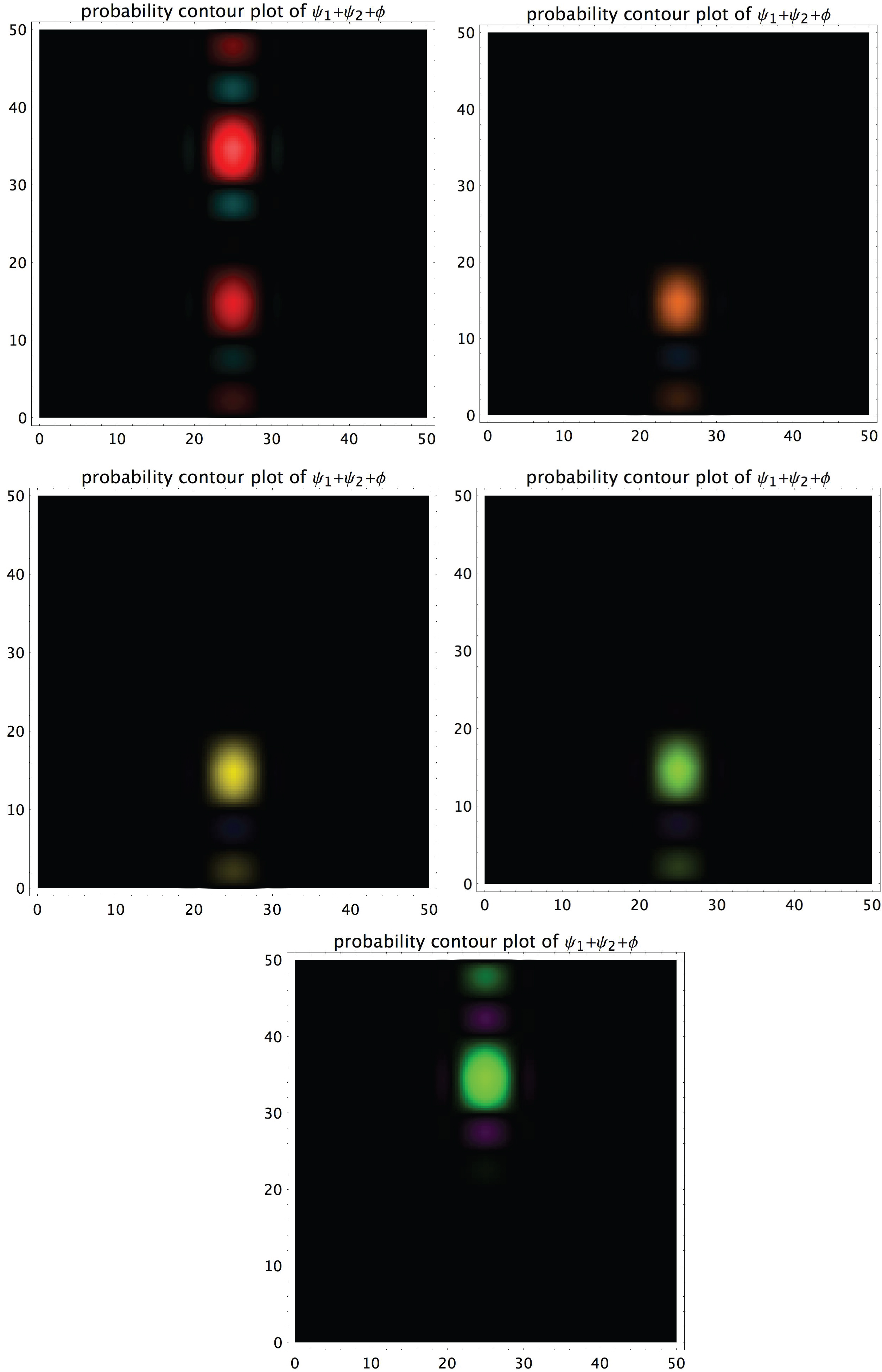
Normalized 3D wave function plots Figure 20:
Figure 21 is the probability contour plot of .
Remark 8 For the robustness and tolerance occurred at control in the nucleus, it needs to discuss their theoretic and computational issues.
Cite [12] to know, perturbation problems always incident at the real laboratory control of particles, optical technique adopted in the physical experiment needs much more delicate control structure setting in system its self and each parameter selection. This induced noise and uncertainties which happened in controlling of particles. For example, in former poster [12], the result is for control of perturbed Klein-Gordon-Schrödinger system as the uncertainties occurred in the electric field, that conclusion is, if tolerance or perturbation is bounded (very tiny) comparing with control variable or quantum system gauge, then control is also valid, feasible and maintain efficiency. It means that quantum control for nuclei is worked under external noise (influence) is small enough. If no boundedness perturbation, then not valid.
At control of macrosystem, the robustness control put at the first place to be considered, such as the policy declaration, large scale complex system cybernetic, scientific management system configuration, the industrial and engineering system confinement, and financial system (rates) adjustment, etc. To say control, it means that there is an objective, a target to achieve, at a macro system, the aim might be quite clear and urgent. An obvious result is desired in a limit time duration. Therefore, robust control is necessary and often to be utilized sufficiently. On the other hand, these robust control concept used in the microsystem, for instance, in the Klein-Gordon-Schrödinger system, it is not so significant than macrosystem. The discussion of robustness as to a quantum system, first, it needs to define what is a robust control meaningful to a quantum particle? second, whether such a robust control is necessary to be surveyed? third, whether robust control worked for control of particles?
As is well known that, there are very famous experiments using the elementary particles, and lots of interesting results had been accomplished in the past century, those physical or chemical experimentation did not be called control of particles, they had been laying on the physics or chemistry experiments in each of their field. Because at those experiments' initial setup, control did not in the mind. Especially, these experiments are for getting the physics results, test fiy the particles detection, interaction and so forth. Modern control theory is proposed at later year in the field of aero engineering for launch of rocket at military purpose. Rapidly, they covered amount of fields, and extended to almost all the scientific areas.
Now, at this paper, let's put the further themes robust control aside, it mainly considers control at nucleus due to it needs us to do control at particles firstly. It is believed that robustness, fault tolerance, perturbation, and uncertainties would be one of the research directions in the future works. With these theoretical and computational results, together with sustainable and successful control of particles at real experiment, at that time, it would be adequate to discuss a great deal problems including robust control, processing control, and many control issues which already appeared at macrosystems, and had sophisticated theory for their application to microsystem.
Conclusions
This work present two dimension control of couple heavy particles in the Yukawa interaction at nucleus. The theoretic analysis and experiment demonstration evident that it is reasonable to execute the quantum controlling with the advanced optical technology. The study would provide a bright perspective for quantum nuclei controlling in realistic meaning. In the future work, the proposed computational approach would be developed to a numerical methodology not only in theoretical study but also in laboratory experiments for a wide class of control problem of quantum system in physical field. Particularly, it can be applied to control of elementary particles at nucleus with a kind of inventing instruments at laboratory.
Acknowledgments
The author really appreciates 258th ACS National Meetings & Exposition 2019.