
International Journal of Optics and Photonic Engineering
(ISSN: 2631-5092)
Volume 5, Issue 2
Research Article
DOI: 10.35840/2631-5092/4526

Article Formats
Applications of OHAM and MOHAM for Time-Fractional Klein-Fock-Gordon Equation
Table of Content
Figures
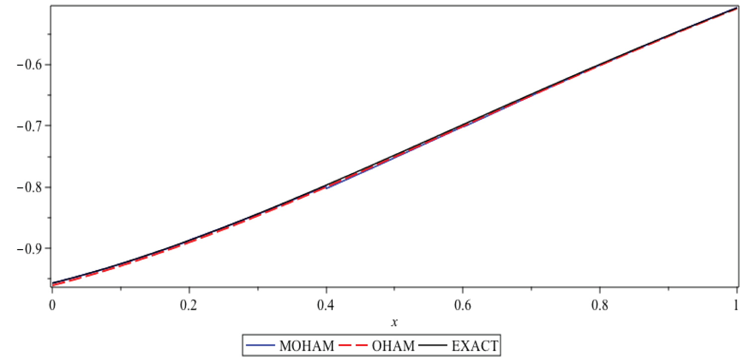
Figure 1: The results of OHAM, MOHAM and Exact....
The results of OHAM, MOHAM and Exact solution for α = 2, at t = 0.6.
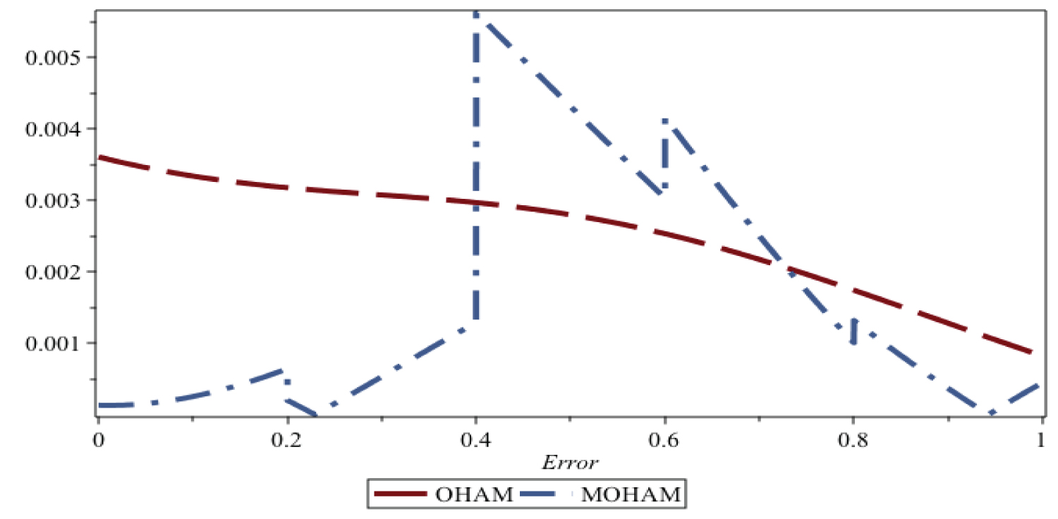
Figure 2: The Absolut Error of OHAM and.....
The Absolut Error of OHAM and MOHAM for α = 2, at t = 0.6.
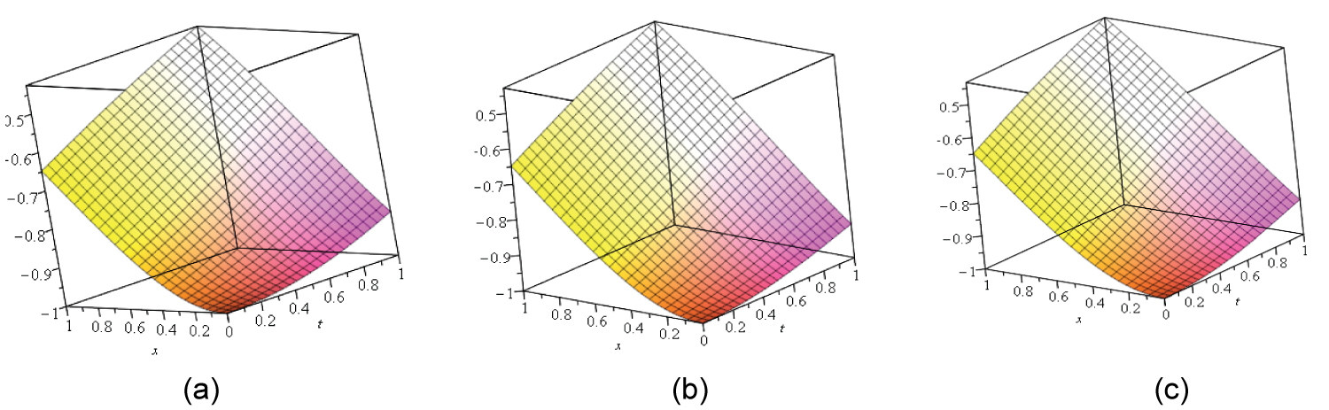
Figure 3: The PLOT 3D of a) OHAM; b) MOHAM....
The PLOT 3D of a) OHAM; b) MOHAM and c) Exact solution for α = 2, at t = 0.6.
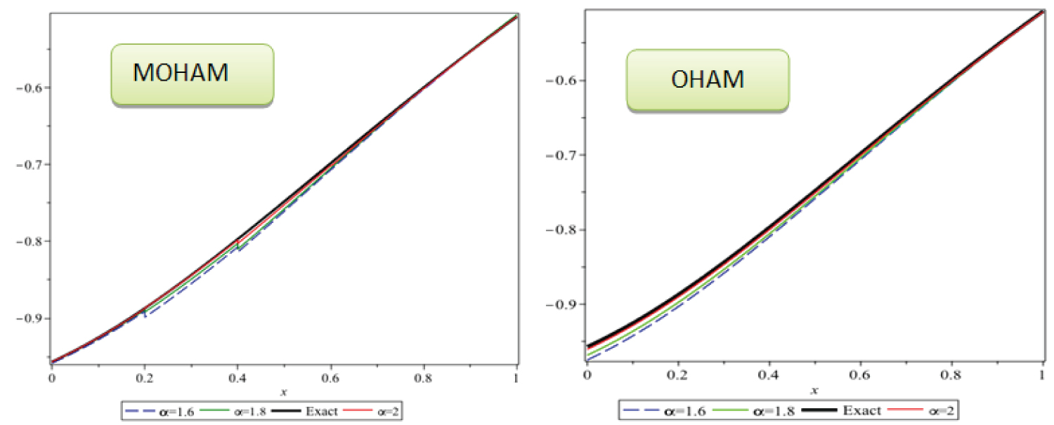
Figure 4: The results of OHAM and MOHAM....
The results of OHAM and MOHAM for different values of α = 2, at t = 0.6.
Tables
Table 1: The value of control parameters ci, for different values of α.
Table 2: Values of control parameters cij.
Table 3: The results of OHAM, MOHAM and Exact solution for different value of x at t = 0.6.
References
- I Podlubny (1999) Fractional Differential Equations. Academic Press, New York.
- MA Abdelkawy, Antonio M Lopes, Mohhamad M Babtin (2020) Shifted fractional Jacobi collocation method for solving fractional functional differential equations of variable order. Chaos, Solitons & Fractals 134: 109721.
- M Jleli, S Kumar, R Kumar, B Samet (2019) Analytical approach for time fractional wave equations in the sense of Yang-Abdel-Aty-Cattani via the homotopy perturbation transform method. Alexandria Engineering Journal 59: 2859-2863.
- KM Saad, Eman HF, Shareef AL, Alomari AK, Dumitru Baleanu (2020) On exact solutions for time-fractional Korteweg-de Vries and Korteweg-de Vries-Burger's equations using homotopy analysis transform method. Chinese Journal of Physics 63: 149-162.
- Mehmet Giyas Sakar, Fevzi Erdogan (2013) The homotopy analysis method for solving the time-fractional Fornberg-Whitham equation and comparison with Adomian's decomposition method. Applied Mathematical Modelling 37: 8876-8885.
- Mehmet Giyas Sakar, Hilmi Ergo¨ren (2015) Alternative variational iteration method for solving the time-fractional Fornberg-Whitham equation. Applied Mathematical Modelling 39: 3972-3979.
- Zaid Odibat (2019) On the optimal selection of the linear operator and the initial approximation in the application of the homotopy analysis method to nonlinear fractional differential equations. Applied Numerical Mathematics 137: 203-212.
- V Marinca, N Herisanu, C Bota, B Marinca (2009) An optimal homotopy asymptotic method applied to the steady flow of a fourth-grade fluid past a porous plate. Applied Mathematics Letters 22: 245-251.
- V Marinca, N Herisanu, I Nemes (2008) Optimal homotopy asymptotic method with application to thin film flow. Central European Journal of Physics 6: 648-653.
- V Marinca, N Herisanu (2008) Application of optimal homotopy asymptotic method for solving nonlinear equations arising in heat transfer. International Communications in Heat and Mass Transfer 35: 710-715.
- N Herisanu, V Marinca, T Dordea, G Madescu (2008) A new analytical approach to nonlinear vibration of an electrical machine. Proceedings of the Romanian Academy, Series A 9: 229-236.
- N Herisanu, V Marinca (2010) Explicit analytical approximation to large-amplitude non-linear oscillations of a uniform cantilever beam carrying an intermediate lumped mass and rotary inertia. Meccanica 45: 847-855.
- S Iqbal, M Idrees, AM Siddiqui, A Ansari (2010) Some solutions of the linear and nonlinear Klein-Gordon equations using the optimal homotopy asymptotic method. Applied Mathematics and Computation 216: 2898-2909.
- S Iqbal, A Javed (2011) Application of optimal homotopy asymptotic method for the analytic solution of singular Lane-Emden type equation. Applied Mathematics and Computation 217: 7753-7761.
- MS Hashmi, N Khan, S Iqbal (2012) Numerical solutions of weakly singular Volterra integral equations using the optimal homotopy asymptotic method. Computers & Mathematics with Applications 64: 1567-1574.
- A Zeb, S Iqbal, AM Siddiqui, T Haroon (2013) Application of the optimal homotopy asymptotic method to flow with heat transfer of a pseudoplastic fluid inside a circular pipe. Journal of the Chinese Institute of Engineers 36: 797-805.
- S Iqbal, AR Ansari, AM Siddiqui, A Javed (2011) Use of optimal homotopy asymptotic method and galerkin's finite element formulation in the study of heat transfer flow of a third-grade fluid between parallel plates. Journal of Heat Transfer 133: 091702.
- NR Anakira, AK Alomari, AF Jameel, I Hashim (2016) Multistage Optimal homotopy asymptotic method for solving initial-value problems. J Nonlinear Sci Appl 9: 1826-1843.
- K Diethelm (2010) The analysis of fractional differential equations. Lecture Notes in Mathematics, Springer-Verlag, Berlin Heidelberg.
Author Details
Jafar Biazar1* and Saghi Safaei2
1Department of Applied Mathematics, Faculty of Mathematical Sciences, University of Guilan, Rasht, Iran
2Department of Applied Mathematics, University of Guilan, Campus 2, Rasht, Iran
Corresponding author
Jafar Biazar, Department of Applied Mathematics, Faculty of Mathematical sciences University of Guilan, P.O. Box. 41635-19141, P.C.41938336997, Rasht, Iran.
Accepted: November 16, 2020 | Published Online: November 18, 2020
Citation: Biazar J, Safaei S (2020) Applications of OHAM and MOHAM for Time-Fractional Klein-Fock-Gordon Equation. Int J Opt Photonic Eng 5:026.
Copyright: © 2020 Biazar J, et al. This is an open-access article distributed under the terms of the Creative Commons Attribution License, which permits unrestricted use, distribution, and reproduction in any medium, provided the original author and source are credited.
Abstract
In this paper the optimal homotopy asymptotic method (OHAM) and multistage optimal homotopy asymptotic method (MOHAM) are applied to obtain an analytic approximate solution to a time-fractional Klein-Fock-Gordon (FKFG) equation. The FKFG equation plays an important role in characterizing the relativistic electrons. The MOHAM relies on OHAM to obtain analytic approximate solutions, it actually applies OHAM in each subinterval and we show that it achieves better results than OHAM over the large intervals; this is one of the advantages of this method which can be used for large intervals and to obtain good results. The convergence of the method is also addressed.
Keywords
Optimal homotopy asymptotic method, Multistage Optimal homotopy asymptotic method, Convergence, Time-fractional Klein-Fock-Gordon (FKFG) equation
Introduction
Fractional calculus (FC) is a part of mathematical analysis that studies the derivation of integrals and derivatives of rational orders [1]. The concept of fractional calculus (integrals and derivatives of any rational order) is established over 300 years ago, and nowadays is a very important subject. Gradually, researchers in different fields of sciences have discovered that fractional differential models have much better descriptors for different phenomena. Fractional calculus has widespread applications of in physics, chemistry, economics, dynamic systems, medical engineering, biological sciences, imaging, etc. On the other hand, physicists Klein, Fock, and Gordon have developed an equation called Klein-Fock-Gordon, which describes the relativity of electrons. This equation is a kind of the wave equation, also relates to the Schrödinger equation, and is a quantitative version of the relation of relative energy and motion. This equation is theoretically similar to the Dirac equation.
Consider the time-fractional Klein-Fock-Gordon equation as follows
Subject to the following initial conditions
Where a and b are real constants and n is a positive integer.
The initial guess to the solution is as follows
Various methods have been developed to obtain approximate solutions of the fractional time differential equations such as, fractional Jacobi collocation method [2], homotopy perturbation transform method [3], homotopy analysis transform method [4], Adomian decomposition method [5], variational iteration [6], and homotopy analysis method [7]. Recently, Optimal homotopy analysis method (OHAM) was proposed by Marinca, et al. [8-12], which was used to obtain analytic approximate solutions for some nonlinear problems [13-17].
OHAM results in to satisfactory solutions on short domains, but when the interval becomes longer, the accuracy of the method decreases, so a new approach was proposed by Anakira, et al. which is called multistage optimal homotopy asymptotic method (MOHAM) that suitable for analytic approximate solutions for large intervals [18].
Finally, the approximate solutions obtained from both methods are compared with the exact solution.
Basic Definitions of Fractional Calculus
In this section, some basic definitions of fractional calculus are explained briefly [1,19].
Definition 4.1: A real-valued function with can be defined on the space , , if there is a real number such
Definition 4.2: The Riemann-Liouville's integral of fractional order for a continuous function with is defined as follows
By considering , , and , the main properties of the operator are listed as follows
Definition 4.3: The fractional-order derivative of in Caputo sense, is defined as follows
Lemma 4.1: By assuming and , the following properties will be valid.
Basic Principles of the Proposed Techniques
A short introduction to the methods that will be used in this research.
OHAM
Let's consider the following fractional equation with the boundary conditions
Where is an independent variable, , and represent, respectively a linear operator, a nonlinear operator, a known function, and an unknown function. Also, shows a boundary operator.
An optimal convex homotopy is constructed as follows,
A deformation equation of zero-order as the following
Where p is an embedding parameter in the interval , is an auxiliary function with non-zero and zero outputs for and , respectively and represents the initial condition of , and is an unknown function. By inserting and 1 into Eq. (13), the following functions are obtained
Therefore, will change continuously from the initial guess to the solution, , to when p increase from 0 up to 1.
By putting into Eq. (13), the initial solution is determined as a solution for the problem
Next, choose an auxiliary function in the following form
Where are called the convergence control parameters, that will be determined later. The auxiliary function can be expressed in other forms see the paper by Herisanu and Marinca [8].
By expanding in Taylor's series about p, the following expansion will be obtained
By putting Eqs. (14-18) into (13), and equating the coefficients of the terms with identical powers of p, one will obtain the governing equation of the initial approximation , given by Eq.(16), and then the governing equation of the first order problem is defined as
And the governing equation of the mth order is defined as
Where is the coefficient of in the expansion of about the embedding parameter p
Solving Eq. (20) gives various approximates solutions , but there exist still m unknowns, auxiliary parameters, in the obtained solutions. It is assumed that the auxiliary parameters , the linear operator L, and the deformation equation of the zero order (16) are appropriately determined in order to ensure the convergence of the series (18) at . Hence, putting Eqs. (14) and (15) into Eq. (18) for gives the solution as
The approximate solution of Eq. (11) can be calculated as
Substitution of Eq. (23) in Eq. (11), results in the following residual
By supposing that , the exact solution will be . However, such a case could not be true for a nonlinear equation. By least squares technique the functional should be minimized
Where a and b are two values relating to the problem in hand. The optimal values of the unknown coefficients can be determined based on the following conditions
In order to get an analytic approximate solution at the level m, the obtained optimal coefficients will be substituted in Equation (23).
MOHAM
Although the OHAM is used to obtain approximate solutions of nonlinear problems. It has some disadvantage in nonlinear problems with large domain. To control this drawback, we introduce in this section a multistage OHAM to obtain the nonlinear problem with long of the domain. A simple way to confirm the validity of the approximate solutions of large T is by dividing the interval in to subinterval as where and utilizing the MOHAM solution on each subinterval. The initial approximation in each interval is given from the solution in prior interval. First, by considering the following initial condition
then we can obtain the initial approximation and the following zero-order equation
Next, we pick out the auxiliary function in the form
Or
Then, the first, second and mth order-approximate solutions can be generated subject to initial condition and the approximate solution as follows,
Substituting Eq. (31) into Eq. (11) yields the following residual
If , then will be the exact solution. Generally, such a case will not arise for nonlinear problems, but we can minimize the function
Where h is the length of the subinterval and the number of subinterval. Now, we can solve Eq. (33) for with changing the initial approximation in each subinterval from the solution in the last point of the prior interval. The unknown convergence control parameters can be obtained by solving the following system of equations
Thus, the analytic approximate solution will be as follows
By this way, we successfully gain the solution of the initial value problem for a large interval T. It should be noted that if the MOHAM expresses the OHAM. One of the benefits of MOHAM is that it provides a simple way to control convergence and regulate convergence region and adjust the convergence region though the auxiliary function involving several convergent control parameters s. In general, this method eliminates the difficulty of finding approximate solutions in large ranges.
Convergence Theorem
If the series (23) converges to , where is produced by Eqs. (16)-(19), and the satisfies the order deformation equation (20), then is the exact solution of (11) [18].
Proof:
Since the series is convergent, it can be written as follows
so, we have
The left hand-side of (20) satisfies
According to (38) and the limit, we have
Applying the linear operator
Eq.(40) can be written as following
So by choosing the optimal , Eq.(41) is converted to the following
Which is the exact solution of the problem.
Solution of the Fractional KFG Equation
We consider one of the nonlinear cases of FKFG equation, for and therefore Eq. (1) becomes
With the initial condition
and the exact solution
Now, we solve Eq. (43) by OHAM and MOHAM.
Solution of FKFG equation by OHAM
Having the linear operator and nonlinear operator
and using Eq. (16), we have
The following problems are resulted from Eqs. (19) - (20)
The First-order problem:
The Second-order problem:
The Third-order problem:
By solving the Eqs. (46) - (48), analytic approximate solutions will be obtained.
In this research, a four terms approximation for is considered. By substituting the solutions of the zero-order, first-order, second-order and third-order into Eq. (43) and using the least squares technique, the parameters are determined for different values of α, as in Table 1.
Solution of FKFG equation by MOHAM
In this section, we utilize MOHAM to Eq. (43). We will consider the auxiliary function as the following
This approach leads to the following sequence of equations
As in OHAM, we obtain two approximate solutions to Equation (43)
By applying the least squares technique, the parameters are determined for different values of α where , and up to as in Table 2.
Approximate solution for is as the following form
From Figure 1, Figure 2, Figure 3 and Figure 4 one can see that the solutions obtained by OHAM and MOHAM are nearly identical with the exact solution Table 3.
Conclusion
In this study OHAM and MOHAM are used to derive an analytic approximate solution for the time-fractional Klein-Fock-Gordon (FKFG) equation. The results obtained from these methods show that MOHAM converges better than OHAM. One observes that the results agree very well with the exact solution. The MOHAM by dividing the interval can obtain better solution than OHAM. As far as the authors are aware, MOHAM has not been used to solve fractional partial differential equations, so far, the method has been tested on fractional-PDE and yields to satisfactory results. The Figures and Tables expose that good results are obtained by MOHAM and more accurate solution as compared to OHAM. The convergence of the method is proved.