
International Journal of Astronautics and Aeronautical Engineering
(ISSN: 2631-5009)
Volume 3, Issue 2
Research Article
DOI: 10.35840/2631-5009/7519

Article Formats
The Aerodynamics of an Oblique Biplane Emirates Aviation University, Dubai, UAE
Table of Content
Figures
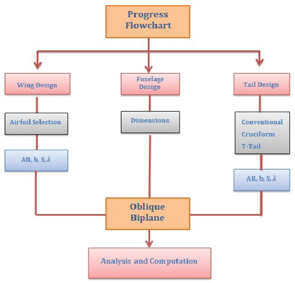
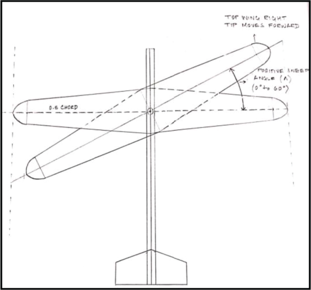
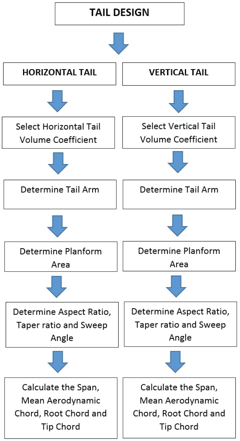
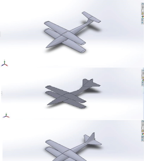
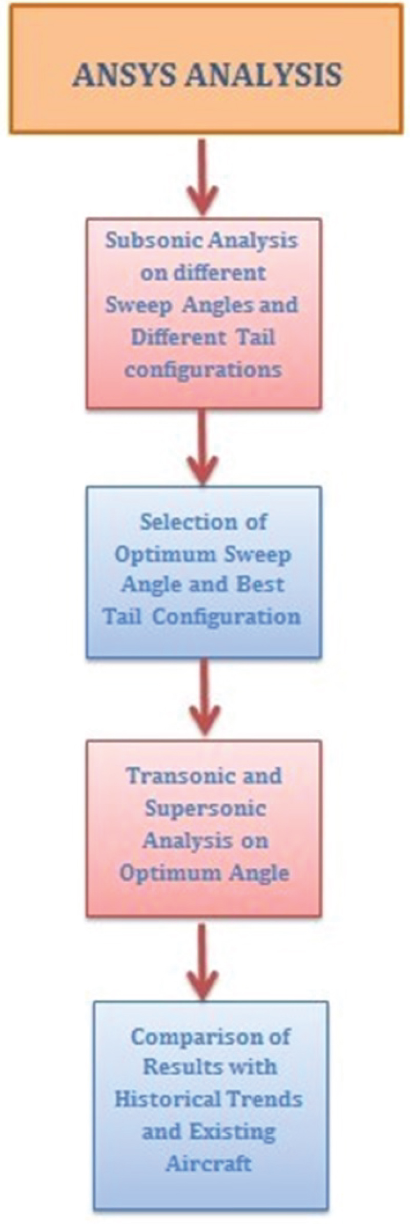
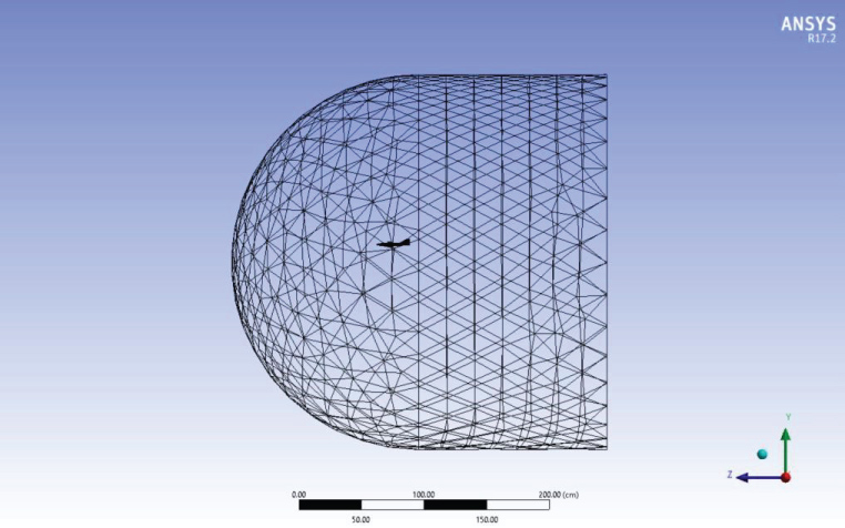
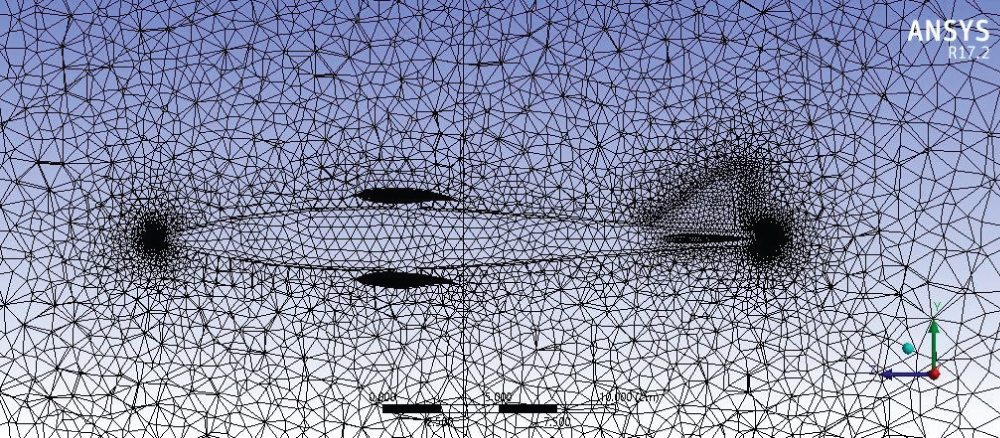
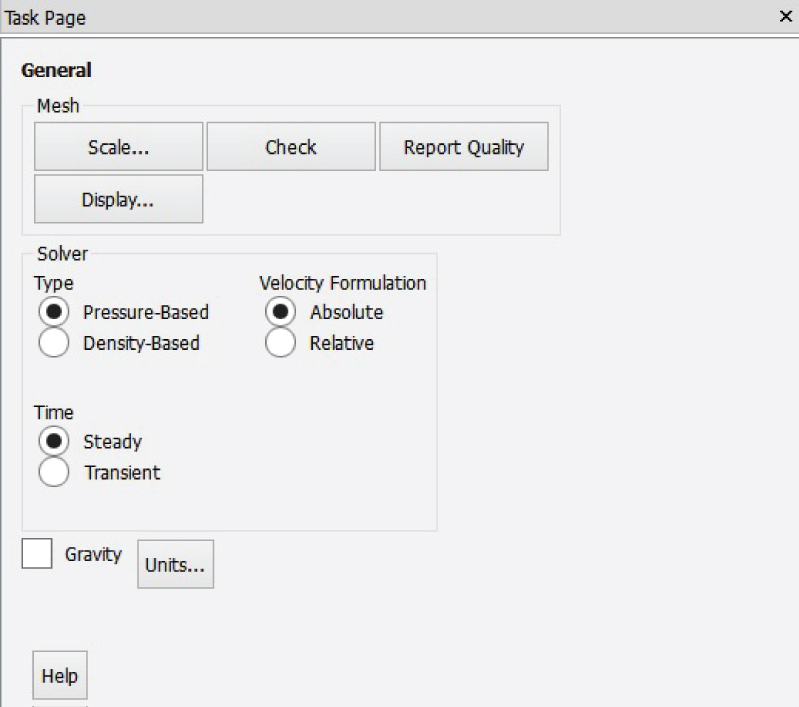
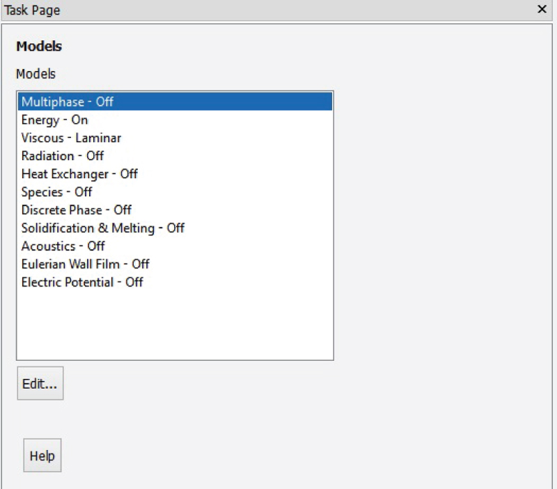

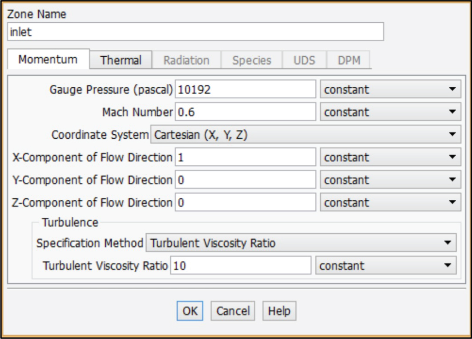
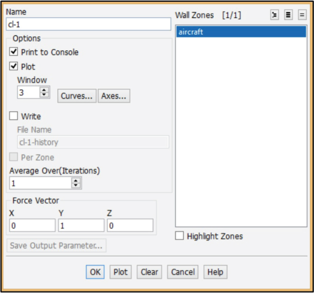
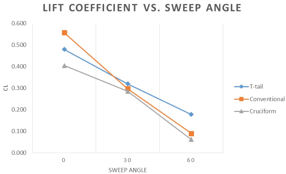
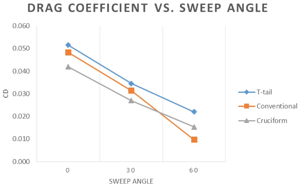
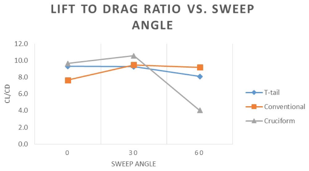
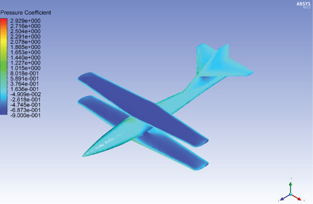
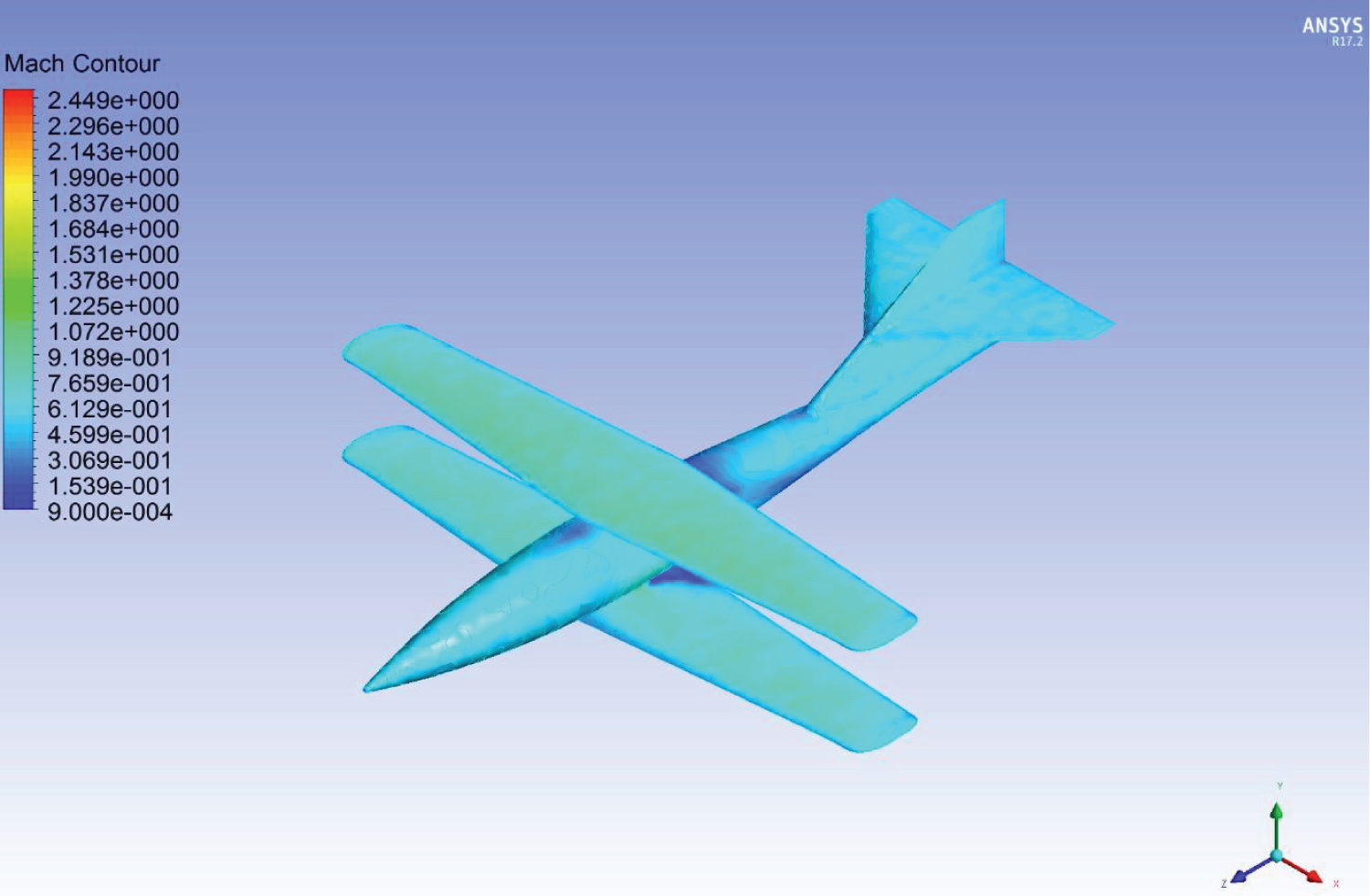
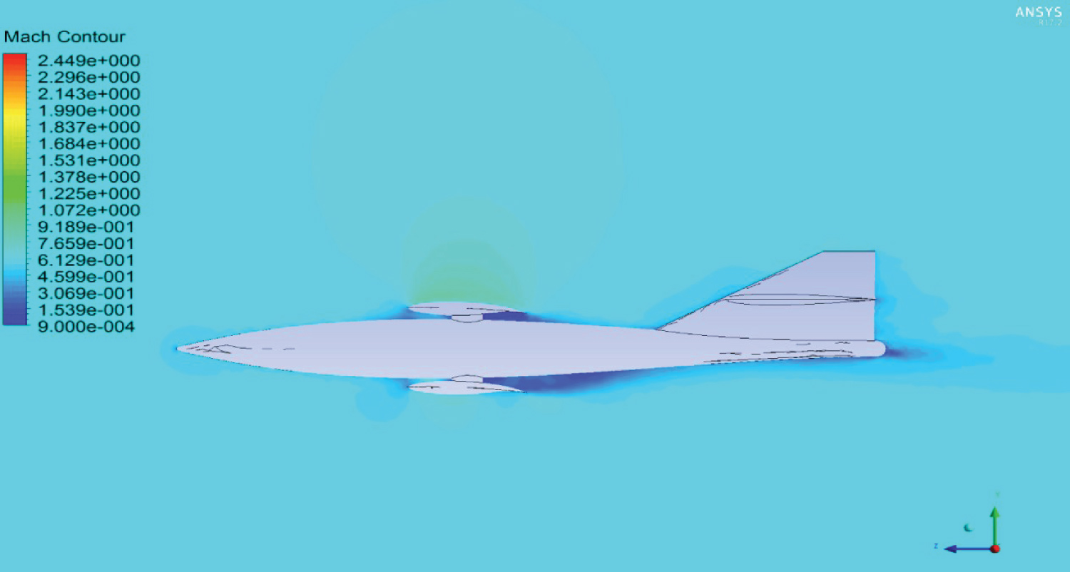
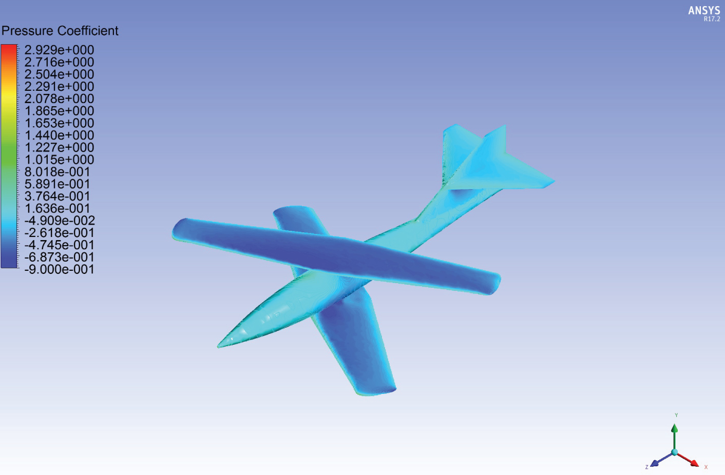
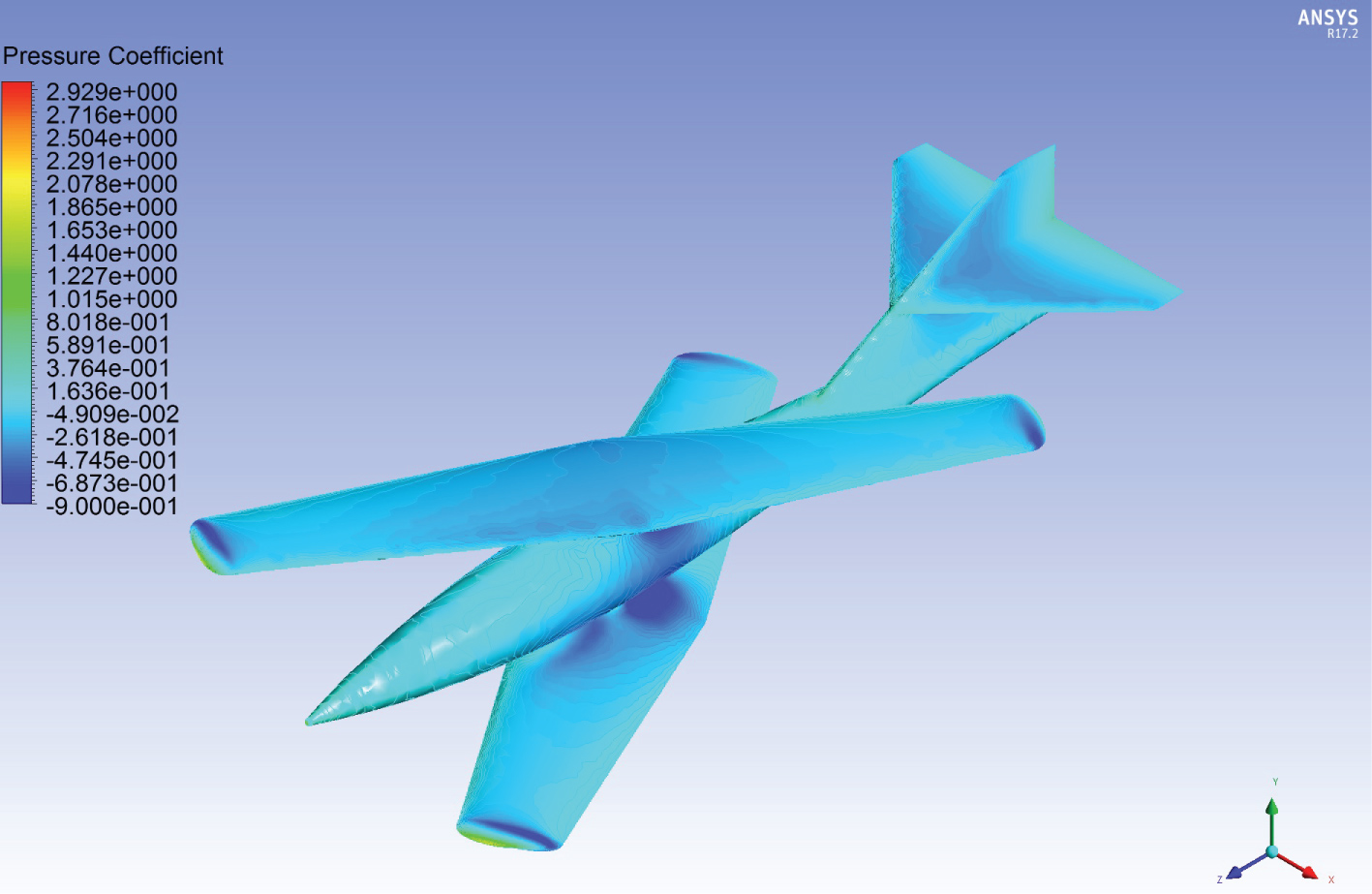
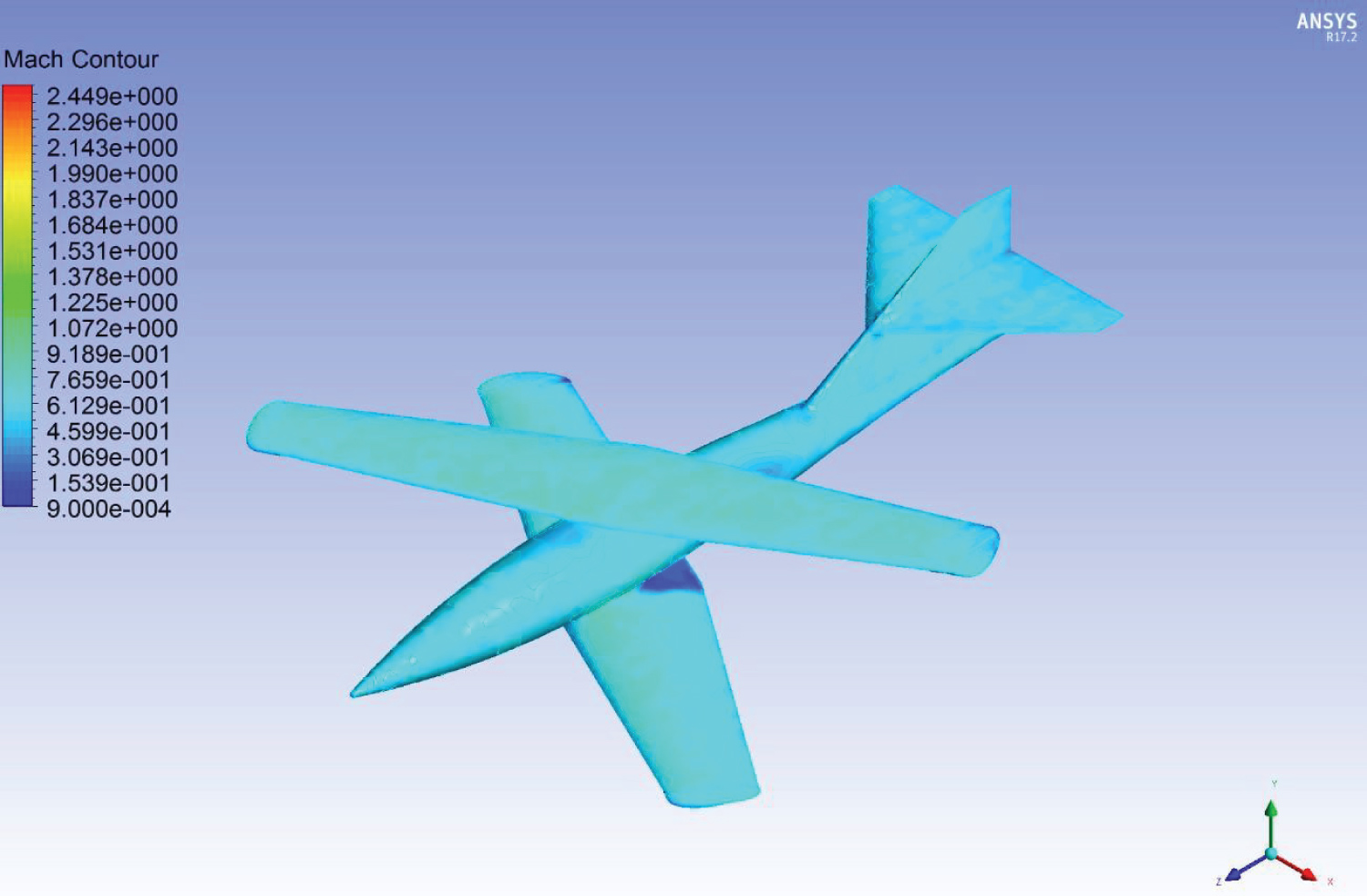
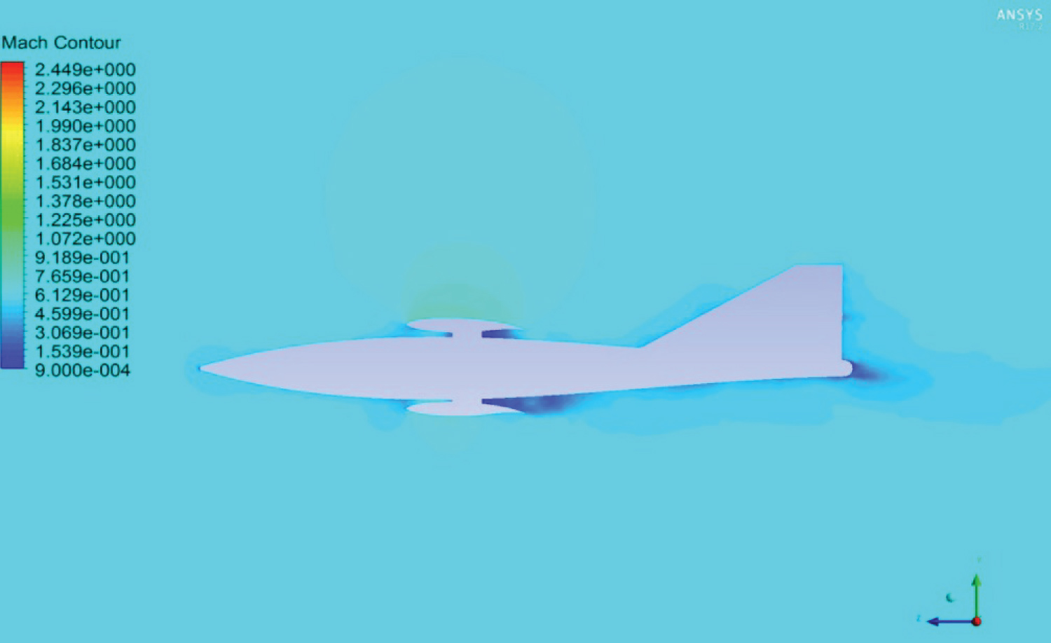
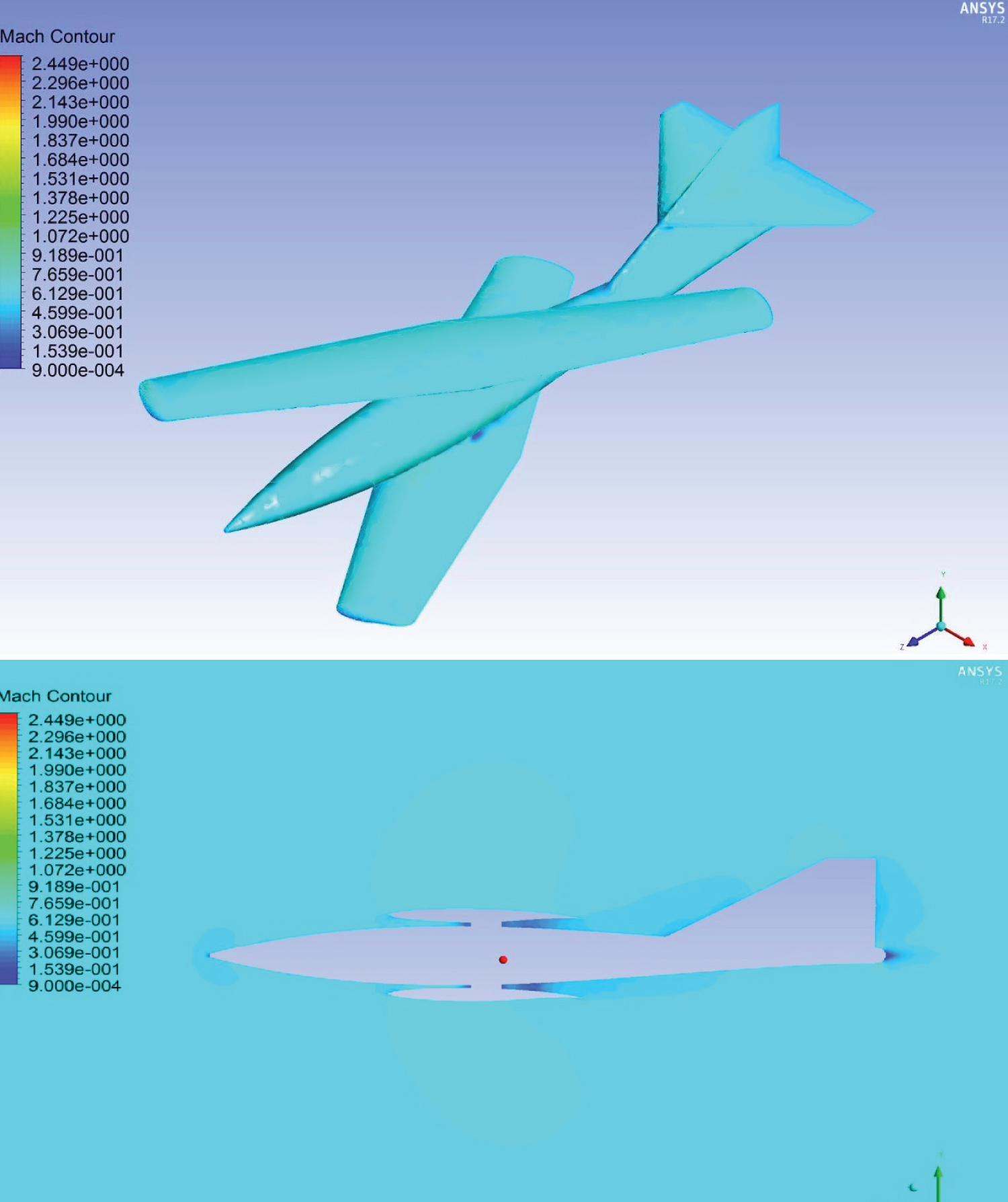
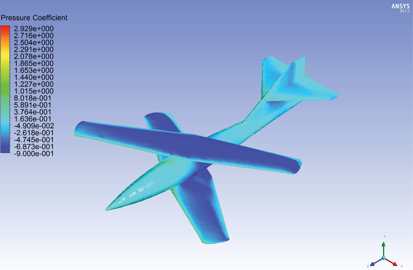
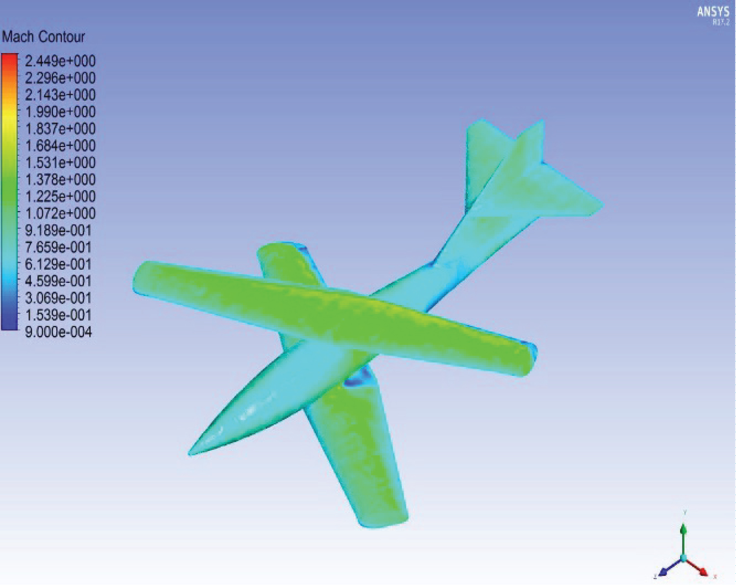
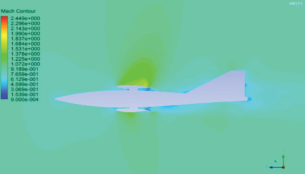
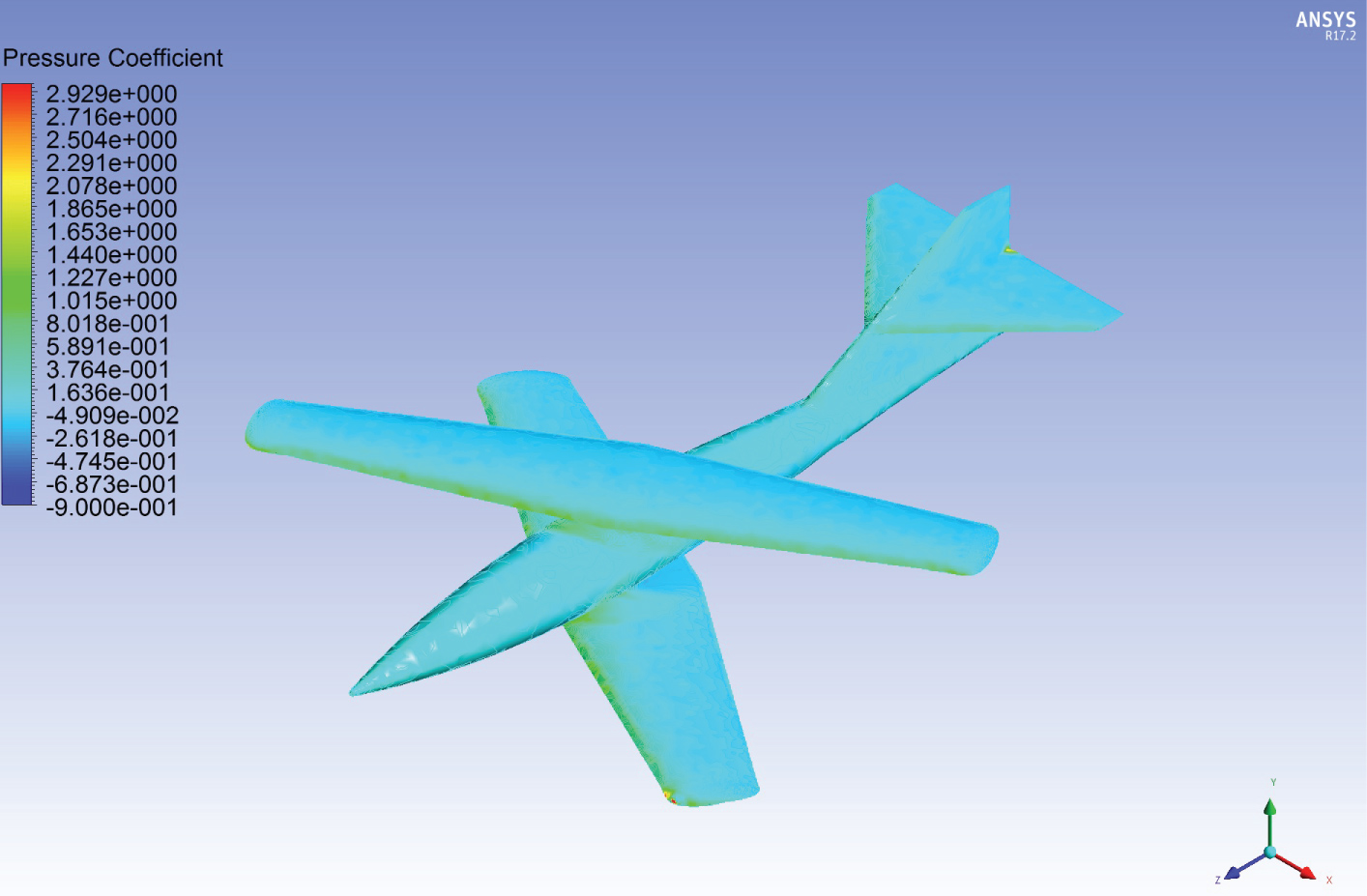
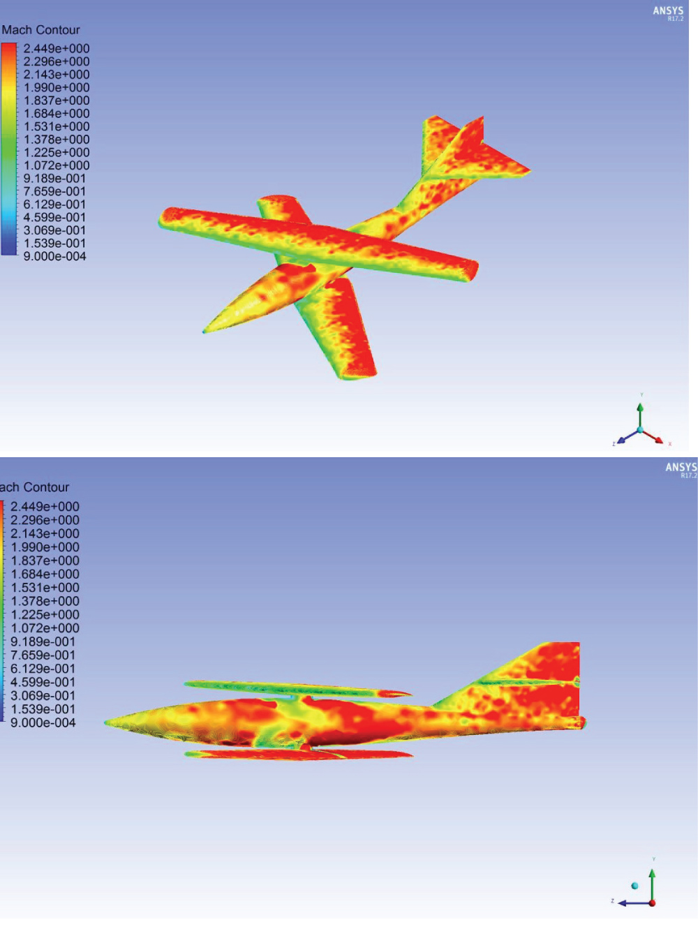
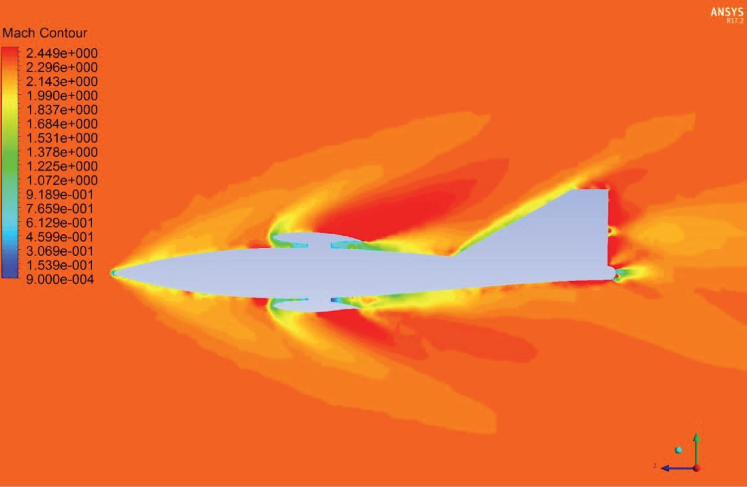
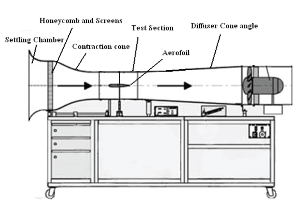
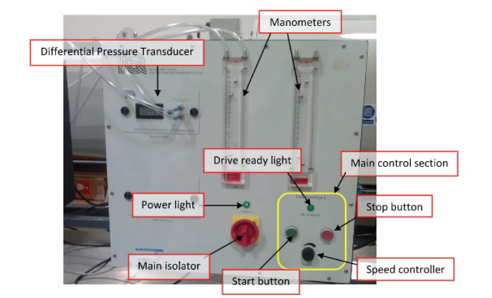
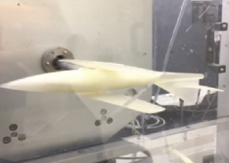
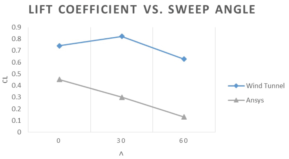
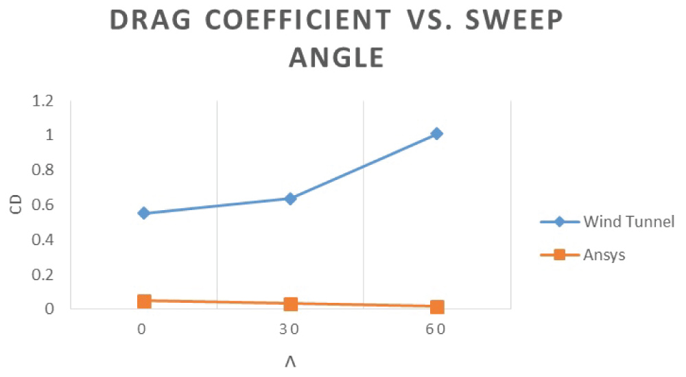
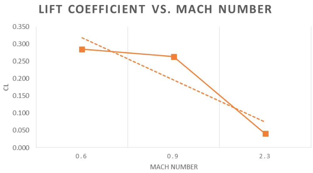
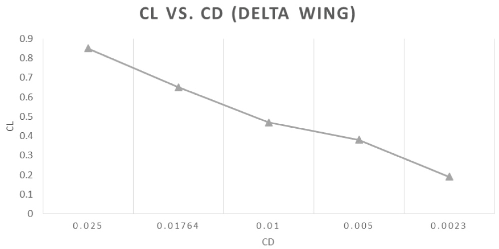
Figure 36: Lift coefficient (CL) vs.....
Lift coefficient (CL) vs. Drag coefficient (CD) for delta wing.
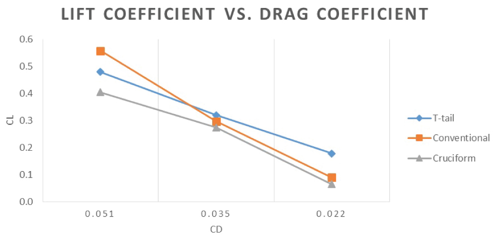
Figure 37: Lift coefficient (CL) vs. Drag....
Lift coefficient (CL) vs. Drag coefficient (CD) for oblique wing.
Tables
Table 1: Wing parameters.
Table 2: Volume coefficients for various types of aircraft.
Table 3: Cruciform tail parameters.
Table 4: Assumptions made for cruciform tail.
Table 5: Conventional tail parameters.
Table 6: Assumptions made for Conventional Tail.
Table 7: Assumptions made for T-Tail.
Table 8: T-Tail parameters.
References
- J Hirschberg M, M Hart D, J Beutner T (2007) A summary of a half century of oblique wing research.
- I Larrimer B (2013) Thinking obliquely.
- (2017) AD-1 Oblique Wing. (1st edn), National aeronautics and space administration.
- Barman S, Shahriar Nafi A, Sayef A (2015) An analysis of aerodynamic forces on an oblique wing.
- Raymer D (2012) Aircraft design. American Institute of Aeronautics and Astronautics, Washington.
- Sadraey M (2013) Aircraft design. (1st edn), A John Wiley & Sons, Ltd.
- D Anderson J (1991) Fundamentals of aerodynamics. (5th edn), McGraw-Hil.
- D Anderson, John (2005) Introduction to flight. (5th edn), Mcgraw Hill, Singapore.
- https://ocw.mit.edu/courses/aeronautics-and-astronautics/16-01-unified-engineering-i-ii-iii-iv-fall-2005-spring-2006/systems-labs-06/spl8a.pdf.
- https://www.princeton.edu/~stengel/MAE331 Lecture4.pdf.
- Richard R Tracy, James D Chase (2012) Laminar flow wing optimized for transonic cruise aircraft.
- Supersonic Aerodynamics (2017) WH Mason.
- https://www.sciencedirect.com/science/article/ pii/S1000936113001143.
- https://history.nasa.gov/SP-468/ch11-3.htm.
- (2017) Unconventional configurations for efficient supersonic flight. Stanford University, US.
- http://article.sapub.org/10.5923.c.jmea. 201502.10.html.
- (2017) Ch10-4.
- https://mhmaberry.wordpress.com/2014/04/02/ a-primer-on-swing-wings/.
- https://www.hq.nasa.gov/pao/History/SP-468/ch11-5.htm.
- http://airfoiltools.com/airfoil/details?airfoil=e417-il.
- http://airfoiltools.com/airfoil/details?airfoil=n0009sm-il.
- Fandavion free fr (2017) Messerschmitt P.1109.
- https://ntrs.nasa.gov/archive/nasa/casi.ntrs. nasa.gov/19870009137.pdf.
- (2017) Thinking Obliquely. National Aeronautics and Space Administration. (1st edn).
- https://www.grc.nasa.gov/www/k-12/airplane/mach.html.
- http://www.dtic.mil/dtic/tr/fulltext/u2/607641.pdf.
- https://www.skybrary.aero/index.php/ High_Altitude_Flight_Operations.
- HM Atassi (2017) Compressibility Effects on Airfoil Lift.
- Supersonic Aerodynamics (2017) California: USAF Test Pilot School.
- Okamoto Satoru (2017) Wind Tunnels. (1st edn), Croatia: InTech, 2011.
- Wind Tunnels (2017) Thermopedia.com.
- https://m-selig.ae.illinois.edu/uiuc_lsat/ lsat_2bulletin.html.
Author Details
Young Hwan Kim, Asma Najib Abdullah*, Awais Khan, Pritam Kumari Devrath, Reem Ahmed Al Ghumlasi and Yasir Nawaz
Emirates Aviation University, Dubai, UAE
Corresponding author
Asma Najib Abdullah, B.Sc in Aeronautical Engineering, Emirates Aviation University, Dubai, UAE.
Accepted: November 21, 2018 | Published Online: November 23, 2018
Citation: Kim YH, Abdullah AN, Khan A, Devrath PK, Al Ghumlasi RA, et al. (2018) The Aerodynamics of an Oblique Biplane Emirates Aviation University, Dubai, UAE. Int J Astronaut Aeronautical Eng 3:019.
Copyright: © 2018 Kim YH, et al. This is an open-access article distributed under the terms of the Creative Commons Attribution License, which permits unrestricted use, distribution, and reproduction in any medium, provided the original author and source are credited.
Abstract
The concept of oblique wings was suggested by R.T. Jones due to its simplified minimum drag solution in supersonic flow [1]. So, what would be the potential advantage of the oblique Biplane. Oblique biplanes have raised bewilderment to whether their application is an advantage or not. The research investigates the aerodynamic modelling of an oblique biplane and analyses its aerodynamic characteristics. The oblique wing is believed to reduce the specific fuel consumption of the aircraft as the wing is adjusting the inclination relative to the free steam, as the aircraft velocity being increased. The aircraft configuration for this study is designed using Solid Works after, which a series of Aerodynamic prediction are conducted, both in the subsonic and the supersonic flow regime using ANSYS Fluent. Through this computational analysis, the impact of various oblique angle shall be tested and the optimum angle will be identified in order to analyze the aircraft stability and aerodynamic characteristics using the wind tunnel with minimum hours experiment. Finally, the obtained computational results are compared to that of the wind tunnel test. The result of this study indicates that the oblique biplane potentially can be the future fighter jet configuration due to its advantage in terms aerodynamics, cost, structural design and weight.
Keywords
Efficiency, Stability, Dynamic characteristic, cost, Oblique wing aircraft, Wind tunnel
Nomenclature
AR: Aspect Ratio; α: Angle of Attack; Cd: Drag Coefficient; D: Drag; Lt: Tail Arm; Ch: Horizontal Tail Volume Coefficient; ARh: Horizontal Tail Aspect Ratio; Sh: Horizontal Tail Area; ARv: Vertical Tail Aspect Ratio; Cl: Lift Coefficient; λ: Taper Ratio; Sw: Wing Area; b: Wing Span; Croot: Wing Root Chord; Ctip: Wing Tip Chord; Sv: Vertical Tail Area; Cv: Vertical Tail Volume Coefficient; : Horizontal Tail Vertical Distance
Introduction
The Germans Luftwaffe had interest about the oblique biplane configuration during WWII due to its distinguished aerodynamic efficiency. Though the Luftwaffe could not complete the oblique winged fighter program "Messerschmitt P1109 [2]" due to the end of war, this idea was adopted by NACA in United States for further implementation and research [2]. Oblique Biplane would offer many advantages at high transonic and low supersonic speeds. However, a variety of uncertainties and technological difficulties associated with this unusual configuration have prevented its application to the operational aircrafts [3]. However, due to the advance of modern technologies, many reasonable solutions were proposed in order to overcome the technical difficulties that this configuration raised.
An Oblique Biplane is capable of sweeping at different angles ranging from 0° for take-off to 60° for cruising. The upper wing, right half, behaves like a forward swept wing and the left half, behaves like a backward swept wing. Vice Versa applies to the lower wing. This opposite rotation of the upper and lower wing around its pivot, cancels out the rolling moment created by each wing and the aircraft remains stable. The advantages of having this configuration is that it distributes the lift over about twice the wing span [1] as a conventional swept wing of the same span and due to its unique aerodynamic features, it shifts the neutral point of the wing and results in reduction of trim drag & the aerodynamic load on the fuselage and empennage. This unique characteristics leads to the increase in the range [4] and speed of the aircraft, hence the better fuel efficiency resulting in the less burdens on the engines to create the required amount of thrust [4]. This study investigates the potential of achieving improved aerodynamic performance and fuel efficiency of the fighter jet at a wide range of oblique angles with the best tail configuration (Conventional, Cruciform, T-Tail). This procedure will assist to identify the optimized wing oblique angle at which the aircraft will provide the better aerodynamic performance during the cruise. This research is targeting to achieve descriptive and applied knowledge about this unique aircraft configuration using computation and experimental approach, completely valid in nature.
Methodology
Progress flow chart- PHASE I
Figure 1.
Fabrication of the aircraft components
For the Oblique wing Biplane in order to ensure the best lift is distributed around the airfoil and high lift is created, the supercritical airfoil SC417 is used. It is desirable to have an airfoil having a greater critical Mach number for high speed aircraft. The purpose of the supercritical airfoil is to increase the drag divergence Mach number.
Solid works
In order to have a reasonable wing length for the required characteristics, to be exact with the design wing geometry formulas were used. An initial sketch was made as shown in the Figure 2.
Wing calculations
The Mean Aerodynamic Chord of the wing was calculated using
The span of the wing was decided based on the size of the wind tunnel test section.
To calculate the wing Planform area, the trapezoidal shape of the wing is considered [5]. Table 1 shows the values.
The steps carried in the calculation of the horizontal and vertical tail parameters is shown in the flow chart of Figure 3. The vertical tail geometries are calculated using the following list of equations:
Aspect Ratio
Taper Ratio
Mean Aerodynamic Chord
Root Chord
Tip Chord
To solve the above equations [6], the aspect ratio, the taper ratio as well as the vertical tail volume coefficient is assumed.
The volume coefficient for all tails is taken from Table 2 for a Fighter aircraft.
The horizontal tail geometries are calculated using the following list of equations:
To solve those set of equations, the aspect ratio, taper ratio as well as the horizontal tail volume coefficient are assumed.
Cruciform tail
The results calculated for the cruciform tail in Table 3 used the assumptions [5] made in Table 4.
The values assumed for the vertical and horizontal tail volume coefficient is taken for a fighter aircraft normal trend.
In addition to the previous mentioned equations, the vertical distance at which the horizontal tail is located in a cruciform tail configuration is found using
Table 3 represents the parameters calculated for a Cruciform Tail.
Conventional tail calculations
The results calculated in Table 5 for the Conventional tail use the assumptions [5] made in Table 6.
Table 5 represents the parameters calculated for a Conventional Tail.
T-Tail calculations
The horizontal tail volume coefficient is reduced by 5% compared to the other tail configurations due to the clean air experienced by the horizontal tail [5]. Moreover, 5% reduction is also applied to the vertical tail volume coefficient because of the end plate effect. Table 7 represents the assumptions made before calculating the parameters for a T-Tail.
Table 8 represents the parameters calculated for a T-Tail.
Aircraft final look
The different Aircraft models are represented in Figure 4 with three different tail configurations to be tested in ANSYS.
Computation and ANSYS analysis
Figure 5 explains the procedure followed when conducting computational analysis on the model.
Generated Mesh for the model
The Mesh is generated as shown in Figure 6 and Figure 7 before running the calculations on the Model in ANSYS. The quality of the mesh highly contributes to the accuracy of the generated results.
ANSYS Fluent Setup and Input Numbers
Step 1: Pressure-based selection
After selecting double precession on the setup window, pressure-based solver is selected in Figure 8. Historically speaking, the pressure- based approach was developed for low-speed incompressible flows, while the density-based approach was mainly used for high-speed compressible flows. In both methods the velocity field is obtained from the momentum equations. In the density-based approach, the continuity equation is used to obtain the density field while the pressure field is determined from the equation of state. On the other hand, in the pressure-based approach, the pressure field is extracted by solving a pressure or pressure correction equation which is obtained by manipulating continuity and momentum equations from aerodynamics analysis.
Step 2: Energy equation
Next step after selecting pressure-based solution is to turn on the energy equation, Figure 9, for further calculation.
Step 3: Material selection
In the setup window, shown in Figure 10, the type of material is selected as "fluid". Next the fluid properties are being selected at the designed altitude. The density is kept as an ideal gas, specific heat coefficient as 1006.43 (j/Kg.K), thermal conductivity is kept constant as 0.0242 (w/m.K) and lastly viscosity is 1.43226e-05 (Kg/m-s).
Step 4: Inlet condition
At the inlet the gauge pressure is kept at 16000 meter which is 10192 (Pa), Mach number is defined as 0.6 and in last the flow direction in Figure 11 is being set up as X-component of flow direction.
Step 5: Lift direction selection
Lastly, lifting body and its direction is selected. Aircraft is kept as a lift creating body and according to the coordinates of the geometry Y-axis is the direction in which lift is being generated as shown in Figure 12. Drag is also defined in a similar manner.
Computational Analysis Results Discussion - Charts
Lift coefficient versus sweep angle
Figure 13 illustrates the change in lift coefficient with change in the sweep angle. According to aerodynamic theory, lift increase with the increase in the Aspect Ratio [7], however, when the aspect ratio decreases contributing to a reduction in the wing-span, the tangential component of velocity increases with the sweep angle. From Figure 13, at 0 sweep angle, the aircraft with conventional tail has its maximum lift coefficient followed by the T-Tail and the least value is for Biplane with cruciform tail. With gradually increasing the sweep angle which results in a reduction in the Aspect ratio, the conventional tail is affected by the downwash of the wings compared to T-Tail and cruciform which results in an abrupt decrease in lift coefficient. At 30 Degree sweep angle T-Tail has the maximum lift coefficient with a value of 0.35 followed by 0.33 and 0.31 for conventional and cruciform tail respectively. The lift coefficient decreases further as the sweep angle reaches to 60 Degree which results in higher tangential velocity on the wing surface. From the figure, there is a dominant fluctuation in lift coefficient value beyond 50 Degree sweep for all tails.
Drag coefficient versus sweep angle
Figure 14 shows the relation between the drag coefficient and the different sweep angles for the different tail configurations. As the sweep angle increases from 0 to 60 Degrees the drag coefficient starts reducing. At 0 Degrees, conventional tails accommodate the highest value of drag at about 0.051, whereas, cruciform shows the lowest value indicated as 0.041. As mentioned previously, the drag keeps on reducing with an increase in sweep angle. At 0 Degrees, the Biplane has the highest wing span. This explains why the three tail configurations experience the highest drag at this sweep angle due to excessive skin friction. As the span starts to change and reduce from 0 to 60, the drag also starts reducing. This is due to the cause that the total drag is directly proportional to the change in the Aspect ratio of the aircraft.
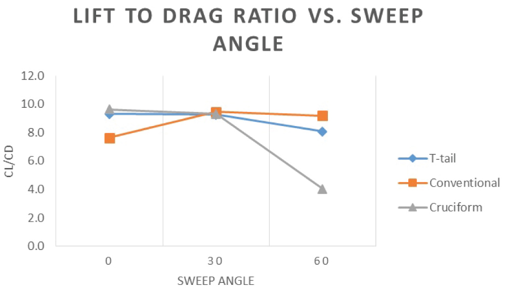
Lift-to-drag ratio versus sweep angle
Figure 15 shows the change in lift-to-drag coefficient versus sweep angle. At zero sweep angle, cruciform and T-Tail has same value for lift-to-drag coefficient whereas the conventional has its least value of around 7.5. From the graph, all the numbers converge to a very near value of CL/CD at 30 Degrees sweep angle for three different tails. At 60 Degree sweep angle conventional tail has the maximum lift-to-drag ratio in comparison to cruciform and T-Tail, this is based on the fact as the sweep angle increase the free stream flow is no longer normal to the leading edge of the wings and will move from tip to root and vice-versa on the surface of the wings till it reaches the trailing edge and leave the surface at an angle. In resultant the conventional tail will experience a uniform undisturbed fluid flow and will have less drag.
Based on the results obtained from ANSYS, the cruciform tail configuration is chosen for further analysis. As stated earlier, the optimum angle is chosen. The Oblique Biplane with a cruciform tail at 30 Degrees sweep angle shows the least value of drag compared to the other tail configurations as well as the highest Lift-to-Drag ratio. This makes 30 Degrees the optimum angle at cruise. The chosen tail at the optimum angle is tested in the transonic and the supersonic flow regime.
Computational Analysis Results Discussion-Mach Number and Pressure Contours
Figure 16 shows the isometric view of pressure distribution over the surface of Biplane at 0 Degree sweep angle with Mach 0.6.Theoretically lift is generated by pressure imbalance [8] on the upper and lower surface of the wings. The pressure coefficient represented on the upper wing is negative indicating the generation of lift by the top surface of the two wings. Stagnation points are observed on some areas of the leading edge of the wing and the frontal area of the pivot as well as the tip of the fuselage nose. At such a point the pressure coefficient is almost 1. The pressure distribution over the surface of the wing is not very disturbed and appears to be relatively uniform until it reaches the trailing edge. This is the case as the wing is moving at a low Mach number so the compressibility effects are not very significant even though the flow is characterised as a compressible flow and not many flow disturbances are observed as there is no fluctuation in the pressure coefficient. Due to the tapered wing [9], the induced drag produced doesn't significantly affect the lift generation [10] at the wing tips and is expected to create very small vortices. The interference drag plays a role at the junction between the wings and the pivot and it causes flow disturbances. The lower wing is affected more to the flow disturbances from the fuselage as well as the pivot laying on top of it. This contributes to an increase in the pressure coefficient.
Looking at the Mach Contour explains the flow pattern and shows the existence of shock waves if any.
In expanding over an aerodynamic shape, the flow velocity increase above the free stream value and if the free stream value is close enough to critical Mach number then the local Mach number will be supersonic in certain regions of the flow. The different colors on Figure 17 represent the difference in the Mach number over the surface of the aircraft. As noticed, the least velocity is observed in the areas where there is a stagnation [8]. Due to the curvature of the wing, the flow starts to accelerate moving upwards to the maximum curvature of the supercritical airfoil. Figure 18 shows the Mach Contour on a transverse plane. The Mach distribution is quite similar on the fuselage surface. At the wings surfaces, there is an abrupt change in the flow Mach number where it reaches to near sonic speed and a normal shock wave [7] is formed over the top surface of the wing, across which temperature, pressure, density of the fluid increase whereas the velocity decreases across the shock wave [7].
30 Degrees sweep angle
As the sweep angle is increased, the lift generation is also affected. The main contribution to the reduction in lift is because the aspect ratio of the wing has reduced by reducing the wing span. As mentioned earlier, the lift changes with the change in aspect ratio. This is because, in aerodynamics the main contributor to the lift component is the velocity perpendicular to the leading edge of the wing. As the sweep angle increases, the perpendicular velocity keeps on reducing, hence a reduction in lift as well as drag. This is seen on Figure 19 and Figure 20 representing 30 and 60 Degrees sweep angle. The stagnation points on the two models are highly predictable. The forward tip of the upper wing and the lower wing is perpendicular to the flow as well as areas like the tip of the fuselage nose and the leading edge of the tail as described earlier for the Oblique Biplane at 0 Degrees sweep. In such areas experiencing a stagnation point, the pressure coefficient is almost approaching 1.
As the flow moves further downstream the cross-sectional area of the fuselage increases and at the same time skin friction drag increases. The inclination in the fuselage nose helps to accelerate flow until it reaches to the wings-pivot area where again the flow experiences a stagnation point. The pressure distribution is uniform on the surface of the wings unless it reaches the trailing edge of the wing where the flow is separated from the surfaces, the disturb flow will propagate further away from the surface in form of vortices.
Figure 21 illustrates the Mach Contour for Biplane at 30 Degree wings sweep angle and Mach 0.6.
Skin friction drag is a major contributor in the flow velocity over the wing surface. Starting from the leading edge of the wings the free stream flow comes in direct contact to the leading edge of the wings, where maximum pressure is felt and the fluid velocity is slowed down. As the air flows towards the trailing edge of the wing, it starts to experience a slight increase in the skin friction drag which causes drag at the rear part of the wings. At the pivot which is a circular mechanism that goes through the fuselage to hold the wings, the flow is perpendicular to its surface which behaves like a wall in front of the flow. From aerodynamics of the circular pivot, the fluid is smoothly moving around the frontal half of the pivot and the flow will be laminar [11] in that region. After that the flow tends to leave the surface and becomes turbulent. This phenomenon is due to the boundary layer separation on the rear half of the pivot. Here the velocity of the flow reduces significantly and the Mach number goes to 0.2. The wing wake influences the horizontal tail. The horizontal tail loses its lift as it experiences the disturbances from the wing. This is because of an increase in pressure over the top surface of the tail which contributes to the reduction in speed as well as the Mach number. The accelerated flow at the wing upper surface results in a weak shock wave. On the upper wing, the Mach number approaches the speed of sound where a shock wave starts to build up on the maximum curvature of the wing surface.
The shock wave tends to be weak due to the non-perpendicular airflow over the wing surface. The higher the sweep angle the weaker the shock wave created at the same Mach number. Figure 22 represents the transverse section.
60 Degrees sweep angle
The flow distribution for the 60 Degrees follows almost the same pattern as that at 0 and 30 Degrees. However, the horizontal tail produces more lift compared to the previous sweep angles. This is because as the wing is swept further, the strength of the vortices reduces due to the reduction in the lift-induced drag [10].
Figure 20 shows the isometric view of Pressure distribution over the surface of Oblique Biplane at 60 Degree wings sweep angle. With increase in sweep angle the wing span decrease and which result is reduction in lift and drag coefficient as discussed earlier. The flow is subsonic with a Mach number ranging from 0.5308 to 0.69 over the surface of wing as shown on Figure 23, except the leading and the trailing edge where the pressure is higher (leading edge) and flow separation (trailing edge). Whereas the tails are in the wake of wings, the disturb flow from the wings will pass through the tails section. Compared to the wings the velocity is lower on the tail surface with a Mach number ranging from 0.39 to 0.6.
The disturbed flow at the pivot will propagate over the Fuselage and will mix with uniform flow coming from the sides of the fuselage.
Compared to 30 Degrees, 60 Degree has a lower normal velocity component on wing surface which results in weak shockwave.
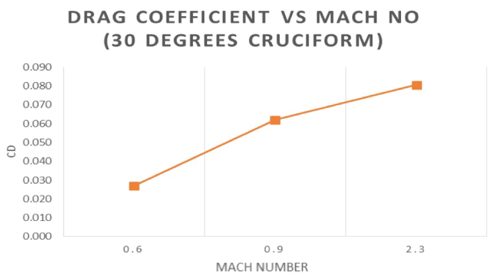
After a series of Subsonic Analysis, the best sweep angle was chosen to be further studied in the Transonic and Supersonic Flow regimes. In the Transonic state, the 30 Degree Oblique Biplane with a Cruciform Tail is tested at Mach 0.9. Furthermore, the same aircraft is tested in Supersonic Flow at Mach 2.3.
30 Degrees (Mach 0.9)
Examining closely the upper and lower wing, the free stream flow hit the leading edge of the wings first where both wings experiences stagnation point with a pressure coefficient of 1.
Transonic flow means both a subsonic and a supersonic flow tend to exist simultaneously on the surface of the aircraft along with the compressible viscous effects of the flow. In a transonic flow regime, the speed increases until it reaches a point where a sonic flow is experienced. This point where the sonic flow exists on the surface is the most critical part of a transonic flow. The Oblique Biplane is Starting our discussion from the upper surfaces of the wings, the Mach distribution contradict from each other, the upper wing right half behaves as forward swept wing and designed using a supercritical wing. This as shown on Figure 24 has contributed in the delaying the onset of shockwaves towards the trailing edge of the wing. However, the pressure coefficient has reduced by a very little increment due to the presence of a shock wave which promotes a supersonic region on the entire surface of the wing.
The lift generated by the plane at Mach 0.9 is satisfactory as long as there is no severe occurrence of strong shock waves.
The delay in the transonic drag rise that causes an increase in the pressure coefficient is an advantage of using the supercritical airfoil which weakens the shock wave on top of the wing.
Left half as backward swept wing and vice versa for the lower wing. From Figure 24, the flow is nearly high subsonic at the most leading edge of both wings with a Mach number ranging from 0.60 to 0.68. After the leading edge the flow start to accelerate over the surface of wing and the transition is obvious from subsonic to transonic and then to supersonic flow. A greater portion of the upper surface wing above the fuselage is covered by shock wave across which pressure, density, temperature and velocity drastically change. In comparison to upper wing, the wing below the fuselage has some disturbed flow around the pivot and fuselage area, where the flow Mach number is relatively decreased to subsonic. As the speed of a fluid approaches the speed of sound, many changes occur to the fluid and this is due to the compressibility effect experienced by the body moving through. Theoretically fuselages are designed to have minimum skin friction drag and the streamlines pass smoothly over the skin of fuselage with uniform Mach distribution. At the pivot, the fuselage accommodates a weak shock wave generated by the lower surface of the upper wing and a strong shock wave produced by the upper surface of the wing below the fuselage. From Figure 25, fluid flow is highly disturbed around the pivot, across which the Mach number drops to subsonic flow again and the flow remains subsonic at some area of the fuselage until it reaches the tail section.
Leading the discussion to Mach distribution over the horizontal and vertical tail as shown on Figure 26, the flow remains transient between subsonic and transonic over the vertical tail of Biplane ranging from Mach 0.7 to 0.85, whereas for the horizontal tail it experiences supersonic flow at its leading edge with a Mach number above one.
On the wing surface the airspeed is faster than the speed of sound hence certain shock waves are created on the surface of the aircraft shown on Figure 26. Since the airfoil used on the wings is a supercritical airfoil, the formation of the shock waves is highly delayed to the trailing edge of the wing.
30 Degrees (Mach 2.3)
Figure 27 shows the isometric view of pressure distribution at Mach 2.3. The force of drag is proportional to the coefficient of drag, to the square of the airspeed and to the air density. Since drag rises rapidly with speed, a key priority of supersonic aircraft design is to minimize this force by lowering the coefficient of drag and reducing the stagnation points over the surface of aircraft [12]. As seen from Figure 27, the surfaces of the aircraft generate a small amount of lift compared to the subsonic and transonic flow regimes. The wing clearly suffers from excessive shockwave formations and the pressure coefficient fluctuates between 1.3 to 1.8.
This is due to the fact that most of the surface of the aircraft is covered with shock waves that increase the wave drag on the aircraft and affect its performance. These locations include the rounded tip of the fuselage nose as well as the leading edge of the wings and the tail. Most of the parts of the aircraft are indicating a positive pressure coefficient greater than unity representing a highly compressible flow. As seen on the Figure 28, most of the aircraft is covered with a supersonic flow as expected.
Here, the flow mechanism changes due to the angle at which the wing is facing the free stream velocity and also due to the flow disturbances that occur around the pivot. As the flow climbs over the surface of the wing, it picks up speed starting from Mach 0.2 at the leading edge to almost Mach 2.2 at the trailing edge. This is shown on the red area over the wings on Figure 28.
Since the horizontal tail does not fall into the downwash region of the wing, it is not affected aerodynamically and can still generate a small amount of lift. This can be shown on the diagram where the velocity increases from the leading edge of the horizontal tail to its trailing edge and at the same time the pressure reduces due to the suction effect that creates the lift.
Oblique shocks are created at the nose of the fuselage, the leading edge of the wing and at the tail of a supersonic aircraft [13]. The aircraft starts with a conical fuselage at the beginning with an increasing inclination until it meets the wing and pivot area. The fuselage nose has a blunt face and this promotes the formation of a weak shock or in other words a curved bow shock. Curved bow shocks [7] form at blunt bodies in a Supersonic flow. This occurs at approximately Mach 2.1 at the nose of the fuselage. The same shock wave occurs at the leading edge of the wing but at a slightly lower value of Mach of approximately 1.8. The area downstream the mid-section of the bow shock represents a sonic flow represented by yellow-green patches on Figure 29. However, as we move further away from the mid-section of the bow shock, the area downstream of the bow shock represents a supersonic flow as shown with orange patches at Mach 2.1. Towards the trailing edge of the wings, a strong oblique shock wave is formed.
Wind Tunnel
Apparatus
The following instruments were used in this experiment are:
• AF-100 Subsonic Wind tunnel, shown on Figure 30: This is an open circuit suction wind tunnel. It permits an assortment of streamlined subsonic examinations including pressure distribution, airfoil tests, limit boundary layer development and other estimation of lift, drag and pitching moment.
• Computer software.
• Pitot probe: Pitot tests are utilized to quantify the pressure upstream and downstream the test model in the test area. They are made of 2 modest channels, which its openings are parallel, and perpendicular to the air stream; the parallel gap measures the aggregate or total pressure and the perpendicular measure the static pressure.
• Aircraft model.
Wind tunnel operation
Start up
The procedure used to operate the wind tunnel initializing frame in Figure 31, is:
1. On control and instrumentation frame switch on the electrical isolator.
2. Speed Control is set to be minimum position (fully anticlockwise).
3. For starting the flow of air, press the green START button.
4. Then, gradually turn the speed control clockwise till desired speed is obtained for the experiment.
Shut down
1. Firstly, turn the speed control fully anticlockwise and then press red button to stop.
Wind tunnel procedure
- Initially to start this experiment, the model needs to be fixed into the test section. The bolts of the test section need to be carefully removed which will detach one of the sides of the test section.
- Model installation, (Figure 32): Firstly, the balance lock of the three component balance must be tightened and locked from the outside. Carefully hold the model with required sweep angle and slowly slide the model shaft into the holder of the model holder in the balance.
- By closing the test section model in it, but if there is no spacing between the ends attached to the walls of the working area, it can cause discrepancies in the measurement of the lift and drag due to the effects of friction forces acting between the wing tips and the test section walls. Therefore, when the airfoil is placed inside the test section a small gap must be left from both ends of the airfoil from the walls of the test section to avoid in accurate results.
• The necessary adjustments are made and are checked for one last time before the test section is closed and the experiment is ready to begin.
• Start the wind tunnel and set the velocity of the air fan at 20 m/s. Take readings of the lift, drag and pitching moment from the computer software.
• Once the experiment is completed reduce the velocity of the airflow to zero. The same procedure is done for other sweep angle.
Results obtained from the wind tunnel
Figure 33 and Figure 34 shows the pattern obtained using correction equation and values obtained from ANSYS. Figure 1 shows the change in lift coefficient with sweep angle. As seen the value of lift coefficient increases at zero Degrees and then increases giving the maximum value for the lift coefficient followed by decrease. The figure shows that the maximum lift given by the wing tunnel model is at 30 Degrees.
Similarly, Figure 34 shows the change in drag coefficient with respect to sweep angle. The graph follows the pattern of increase in drag with increasing sweep angle.
The highest drag coefficient value is at 30 Degrees. As seen on both Figure 33 and Figure 34, the lift and drag created the Oblique Biplane on ANSYS generates lesser lift and hence drag. This is because the wind tunnel computation was carried at sea level; however, the ANSYS computation was carried at an altitude. With an increasing altitude, the air density reduces and hence the aerodynamic forces since they are directly proportional to each other.
In Figure 34, the drag value of the Oblique Biplane at 30 and 60 Degrees is increasing. This is because the wing on the 3D printed model started fluttering as the speed of air was increased. This caused a fluctuation in the drag value. However, if this issue was resolved, the drag should follow the same trend as that in ANSYS shown on Figure 34. The drag should reduce with increasing sweep. Due to the same issue the value of the Lift was also affected.
Chapter 9: Comparison of Results
Lift coefficient vs. Mach number for 30 degree oblique biplane with cruciform tail
Figure 35 shows the effect of increasing the Mach number of the Oblique Biplane at 30 Degrees sweep angle and a cruciform tail. As the Mach number increases the compressibility effects become significant due to the changes in density. The aerodynamic forces acting on the aircraft highly depend on the changes in density at different flow regimes. The compressibility effect becomes more sincere as the speed of the aircraft increases. The fluctuations and disturbances that occur as the aircraft increases its speed and in turn the Mach number can create sudden shock waves that have a direct effect on the lift and drag.
At Mach < 1, the compressibility effect can be ignored. So from Figure 35, at Mach 0.6 and 0.9, the compressibility effects are ignored and as seen there is no significant change in the Lift.
At Mach > 1, the compressibility effects become very significant and the density changes faster than the velocity of the aircraft. This causes a severe change in the lift generated by the aircraft as seen at Mach 2.3 on Figure 35.
Lift-to-Drag ratio: Delta wing vs. Oblique biplane
Figure 36 illustrates the change in the lift coefficient with change in drag coefficient for delta wing. The cross-sectional area of a delta wing is higher compared to the Oblique wings which results in induced drag of the lifting wing. By comparing CL versus CD of delta wings and Oblique wings on Figure 36 and Figure 37, it is seen that they follow the same trend, as the lift coefficient decreases; the drag also decreases with it.
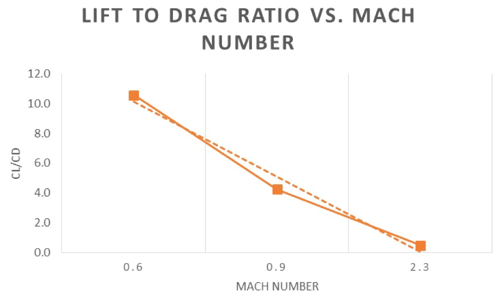
Lift-to-Drag ratio vs. Mach number: Variable sweep wing vs. Oblique biplane
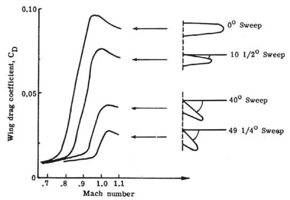
As shown in Figure 38, the Oblique Biplane using a Cruciform tail follows the same general trend of variable sweep wings in Figure 38. The drag remains almost constant at low subsonic speed however it shares a significant increase as the flow turns into transonic and eventually supersonic as shown in Figure 39.
Lift-to-Drag ratio vs. Sweep angle: Swing wing vs. Oblique biplane
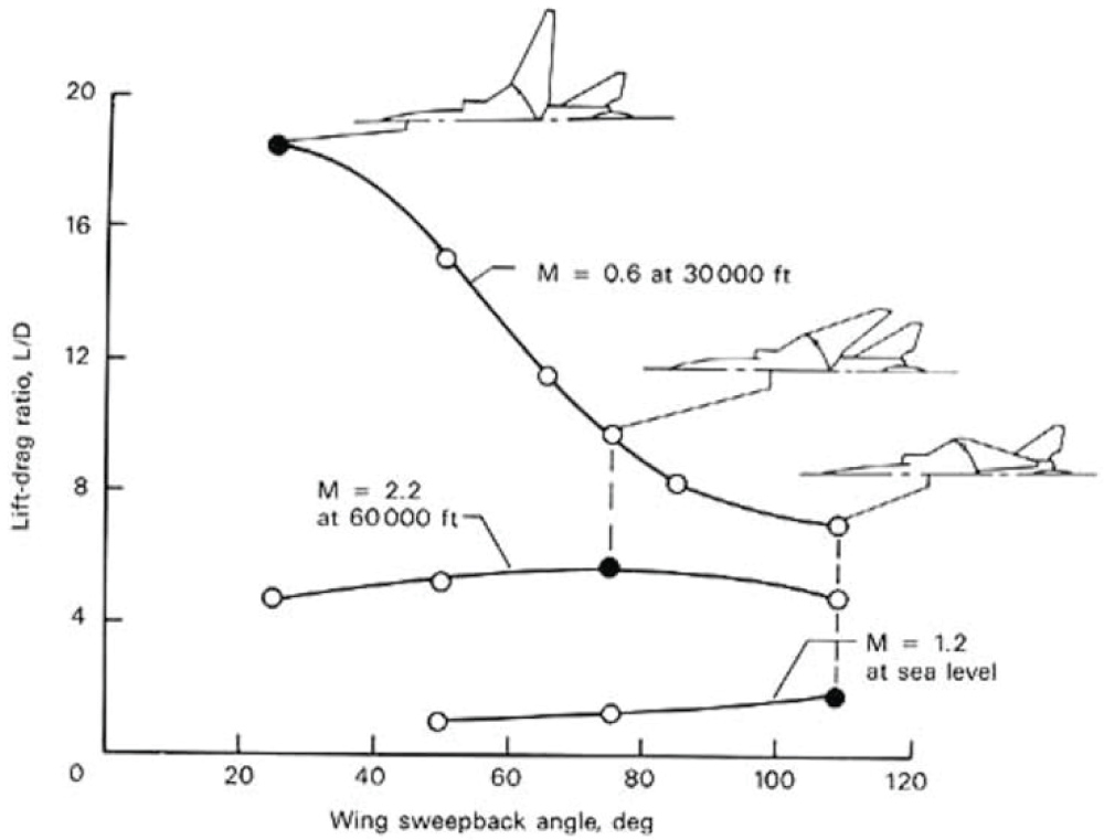
The Lift to Drag ratio represented on Figure 40 follows the same trend as that obtained from the Oblique Biplane. The Lift to drag ratio increases as the sweep angle increases from 0 to 60 Degrees. For a variable swept wing, the flow parallel to the wing has no effect on it, however, as the sweep angle is increased, the flow perpendicular to the wing gets slower (lesser) than the actual airflow [14], it consequently exerts less pressure on the wing. Therefore, the lift to drag ratio of the Swept wing reduces with an increasing sweep angle [14]. The same trend is followed by the Oblique Wing on Figure 41 at which the Lift to Drag ratio reduces with an increase in the sweep angle for a T-Tail and a Cruciform tail however, By comparing the two graphs for the variable swept wing and the Oblique wing, it is noticed that the Oblique wing has the highest value of lift to drag ratio at 0 Degrees which is the same case with a variable swept wing.
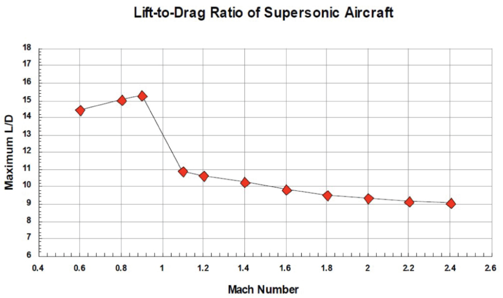
Lift-to-Drag ratio vs. Mach number: Supersonic aircraft vs. Oblique biplane
There is a huge emphasis on the aerodynamics of the flow when it comes to supersonic Mach numbers. As shown on Figure 42, the Lift-to-Drag ratio at subsonic speeds is higher compared to that seen in supersonic. Figure 43 shares the same trend as that in Figure 42. Typically, the Lift-to-Drag ratio of a supersonic aircraft is half that of a subsonic one [15-32]. However, since the size of the model on which the test was conducted is very small, it is expected that the lift and drag values will be lesser than that of an actual, bigger model because of the size limitation.
Conclusion
The purpose of this research was to investigate the potential of achieving improved aerodynamic performance and efficiency of flight at a wide range of oblique angles with different tail configurations (conventional, T-Tail, cruciform) on an Oblique Biplane.
It is clearly seen from the results obtained that, Oblique wing has reduced drag coefficient as the sweep angle increases in comparison with a conventional symmetrically swept design. Fundamentally, this is due to the increased length of an Oblique wing, which is twice as long as a symmetric wing. Moreover, the research shows that Oblique wings tend to perform better at high subsonic or transonic Mach numbers and very low supersonic Mach numbers due to the formation of excessive shock waves at higher Mach numbers. It is also found that for higher Mach numbers, 30 degrees is not very sufficient and will be a victim of excessive wave drag. Increasing the sweep angle will improve the performance at high subsonic and supersonic flow regimes.
Based on the tabulated results, the model with the cruciform tail configuration is chosen as the most effective candidate for the aircraft because of its adequate and relevant aerodynamic performance.
It is believed that reducing the effect of drag and shock waves occurrence on the surface of the Oblique Biplane will render the Aircraft fuel efficient. The Oblique Biplane can be the future fighter jet aircraft because of its high value performance in terms aerodynamics, cost, structural design and weight.