International Journal of Astronautics and Aeronautical Engineering
(ISSN: 2631-5009)
Volume 6, Issue 1
Original Article
DOI: 10.35840/2631-5009/7547

Article Formats
Synthesizes Optimal Conduction Law for Radio Self-Guided Missile Class
Table of Content
Figures
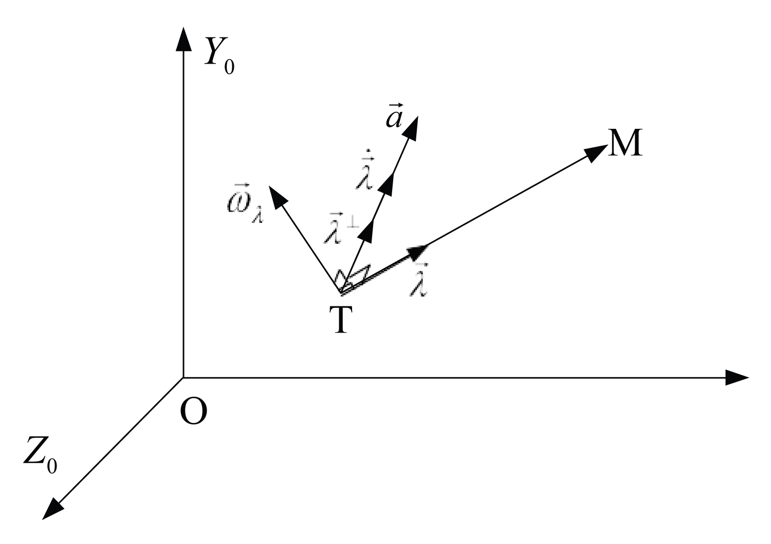
Figure 1: The required acceleration vector direction of....
The required acceleration vector direction of the rocket in space.

Figure 2: The lead trajectories of the two laws.....
The lead trajectories of the two laws lead to survey.
References
- Anh PTP, Vu N, Lai PT, Vinh NQ (2019) Sliding mode based lateral control of unmanned aerial vehicles. Procedia Computer Science 150: 78-87.
- Yanushevsky R (2008) Modern missile guidance. Taylo & Francis Group LLC, CRC Press.
- Zarchan P (2012) Tactical and Strategic missile guidance. The Americal Institute of Aeronauties and Astronautics Inc, 239.
- Hieu NS, Tuan DT, Trung VA (2020) A computational method for optimal midcourse guidance law with impact gust wind. Journal of Mechanical Engineering Research and Developments 43: 388-399.
- Xiaotian C, Wang J (2019) Optimal control-based guidance law to control both impact time and impact angle. Aerospace Science and Technology 84: 454-463.
- Youan Z, Ma G, Liu A (2013) Guidance law with impact time and impact angle constraints. Chinese Journal of Aeronautics 26: 960-966.
Author Details
Vuong Anh Trung*
Air Defence-Air Force Academy, Son Tay, Ha Noi, Vietnam
Corresponding author
Vuong Anh Trung, Air defence-Air force Academy, Son Tay, Ha Noi, Vietnam
Accepted: March 10, 2021 | Published Online: March 12, 2021
Citation: Trung VA (2021) Synthesizes Optimal Conduction Law for Radio Self-Guided Missile Class. Int J Astronaut Aeronautical Eng 6:047
Copyright: © 2021 Trung VA. This is an open-access article distributed under the terms of the Creative Commons Attribution License, which permits unrestricted use, distribution, and reproduction in any medium, provided the original author and source are credited.
Abstract
The paper considers a method to build optimal conduction law solve the problem of local optimization of the omniscient form based on Letov-Kalman approach. The obtained optimum lead law is similar to the traditional proportional lead law, but the ratio coefficient varies with missile-target distance. The law of conductivity can be realized for the active radio self-guided missile class.
Introduction
In the field of rocket guidance, number of studies suggests different laws of conduction. The law of proportional approach with the fixed coefficients (traditional proportional conduction law) has been widely applied since its high realization ability. However, the paper [1,2] has shown that this lead law has many limitations in the case of self-guided missiles with maneuverable targets. Therefore, the law of conduction has been continuously studied to find a new law of conduction that can improve the quality of missile guidance in the case of mobile targets [3].
Optimized Control Algorithm According to Local Standards
Consider a linear control system with a defined structure as follows:
Where: - the output state vector of the system
- the systemic noise vector of the Gaussian white noise with the mathematical expectation of 0;
u(t)- control signal vector
Fy, By -Control efficiency matrix.
The index function of the local quality:
Which: XT - the request state vector
Q- matrix of penalty coefficients according to accuracy at time t
K- matrix of the penalty coefficients according to the magnitude of the control signal
Solving the problem of finding optimal control signals for system (1) and slab (2) by Bellman dynamic planning method.
Equations of State Describe Self-Conduction Kinetics in Space
The spatial self-conducting geometry is described by the vector equation
Which: , is the total acceleration vector of the target and missile is the unit vector of missile-target distance vector with
To describe the coordinates of the vectors in the fixed ground coordinate system (inertial coordinate system) we use vectors. The corresponding state silk is as follows:
The state vector describes the instantaneous state of the line of sight:
Put:
In which: O3- is a square matrix of order 3, including only zeros; I3 is a 3 × 3 unit matrix.
From equations (5) to (7) we have self-conducting geometry described in terms of equations of state
Select the Optimal Slab and Determine the Optimal Lead Law
Select the optimal slab as follows:
In which: qh > 0 is the penalty coefficient according to the instantaneous slip; ku > 0 is the penalty factor for the total acceleration (or overload) required up to time t.
Vector depicts the desired state of sight
Put:
Then the (9) equivalent of the slab
When synthesizing the conduction law in the absence of information about the target acceleration, the target acceleration can be considered as an unknown random effect. The state equation without the impact of the target acceleration has the form
Applying optimal control algorithm for system (13) and local criteria blade (12) we have
From (5) and (14) we have optimal lead law corresponding to the criterion (9) or (12)
The symbol is the vector of the angle of rotation of the line of sight, we have and
With are unit vectors of and respectively
From (16) we have perpendicular to each other and set up the perpendicular coordinate system in space, so we can describe the direction of the required acceleration vector of the name. The rocket corresponds to the law of missile guidance (15) as shown in the Figure 1.
According to [4] the line of sight kinetics is described by the equation
In which: are the projections of the target acceleration vector, the missile is perpendicular to the line of sight and lies in the self-guided plane.
From the picture and according to (16) we have
Replace (18) into (17) and transform we have
In which: is the speed at which the missile approaches the target
According to [5], the instantaneous slip h of the self-conductive process is determined by
Where ΔV is the magnitude of the vector
The instantaneous slip (h) of the self-conduction process is proportional to the rotation speed of the line of sight so allowing the self-guided control ring to ensure that the instantaneous slip h → 0 will correspond to the control of the rocket maneuver so that ωλ → 0. Equation (19) shows that when the missile is self-conducting according to the law (15), the self-conducting control ring corresponds to the first order of inertia stage with the time constant:
When a missile attacks a mobile target, the total active self-driving time is usually very short. Therefore, to ensure the required slip at the meeting point, we set a requirement to limit the transient time of the self-conducting control ring right from the start of self-conduction:
Tcp- allowable limit of self-conductive control loop time constant.
From (21) and (22) we have the boundary condition of (22) being equivalent
For (qh, ku) choose according to (23) then the law of leading (15) becomes
The law of conductivity (24) ensures that the transient time constant of the self-conductive control loop is equal to the limit of the permissible value. Unlike the traditional proportional conduction law, this law of conduction has a proportional coefficient that decreases with distance and depends on the time constant limit [6].
The Simulation Results Evaluate the Optimal Lead Law
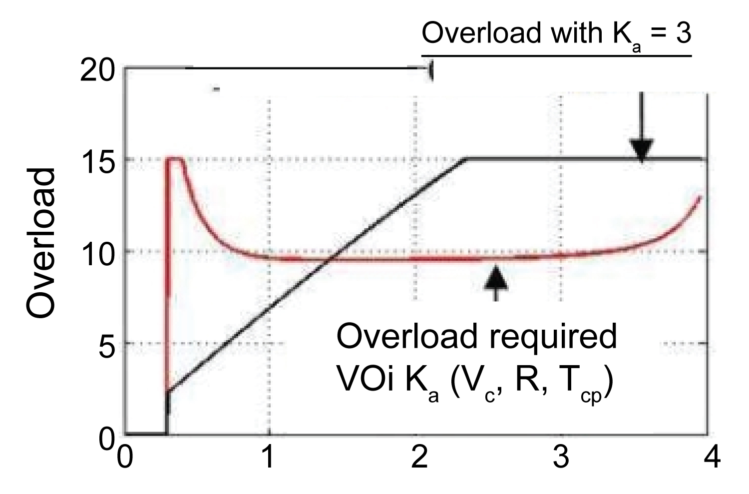
Simulations are performed with traditional proportional conduction law (coefficient K = 3) and optimal conduction law (24) under the same conditions: [km]; target overload nmt = 9, flight time tq0 = 0.3 [s] Figure 2, Figure 3 and Figure 4.
Comment
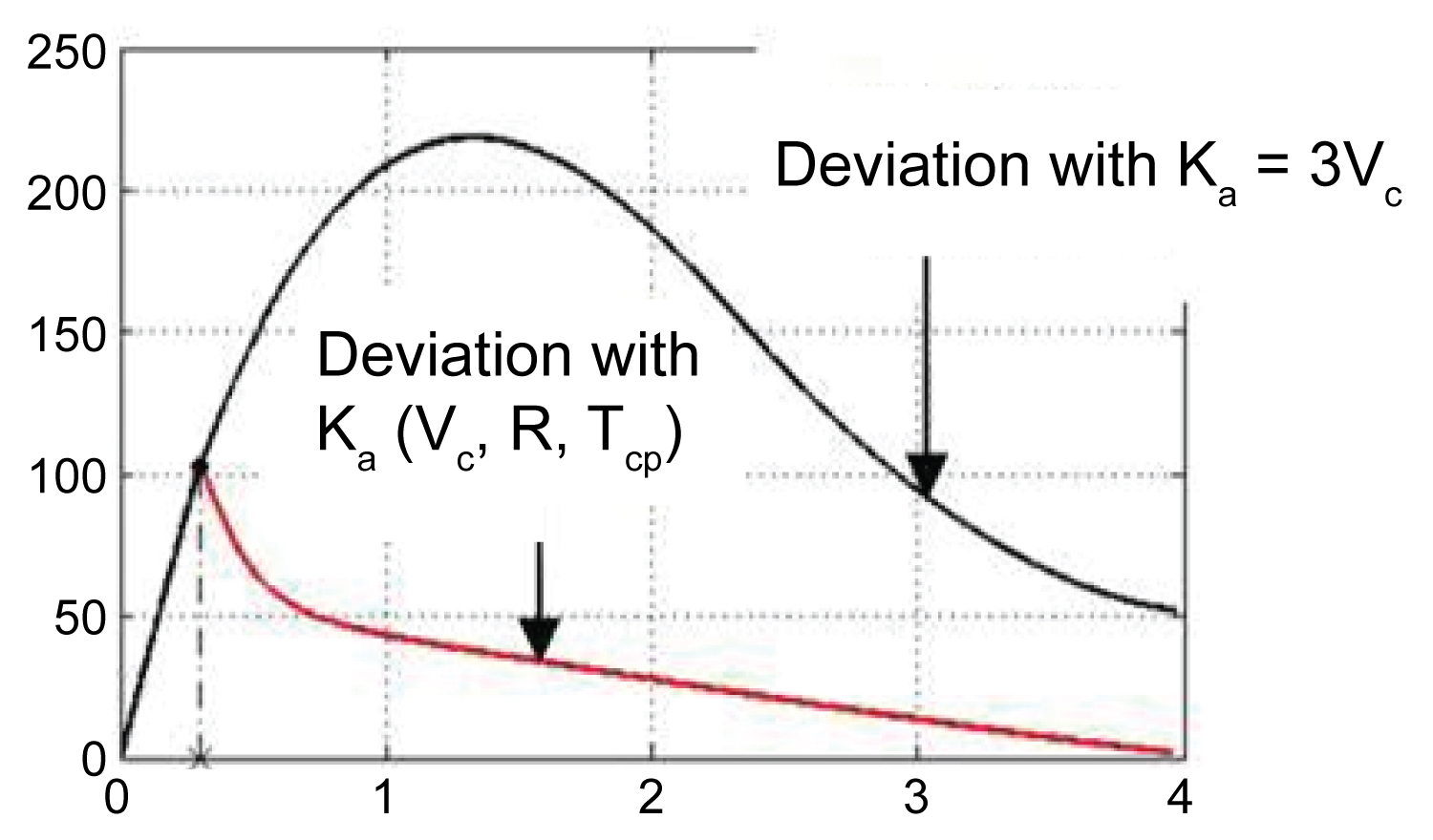
• When the target is strongly mobile, the slip at the meeting point of the orbit corresponding to the law of conduction (24) is significantly smaller than the slip at the meeting point of the conduction trajectory corresponding to the traditional proportional conduction law.
• With traditional proportional conduction law, at the beginning of self-conductivity, the required missile overload is of small value so that the initial slip is not quickly eliminated from the start thanks to the maximum effective overload of the name fire.
• With the law of conductivity (24), because slip is always required to reduce quickly with limited transition time, the day from the start of self-conductivity, according to the requirements of the law of conductivity, the missile using the overload is maximized to quickly reduce the initial slip. Therefore the initial slip is reduced faster and the slip at meeting point is guaranteed to be small enough as required.
Conclusion
The survey simulation results show that the obtained optimal conduction law meets the quality requirements of the self-conductive control loop and is more effective than the traditional ratio approach law when the target is maneuverable. This law of conductivity can be applied to the active radio self-guided missile class, which helps to improve the conductivity of these missiles in aerial combat with highly maneuverable flying targets.