
International Journal of Magnetics and Electromagnetism
(ISSN: 2631-5068)
Volume 4, Issue 1
Research Article
DOI: 10.35840/2631-5068/6511

Article Formats
Three Dimensional Time Domain Simulationof the Quantum Magnetic Dipole
Table of Content
Figures

Figure 1: A quantum torus that is 70 angstroms in diameter;...
A quantum torus that is 70 angstroms in diameter; the tube is 10 angstroms in diameter.
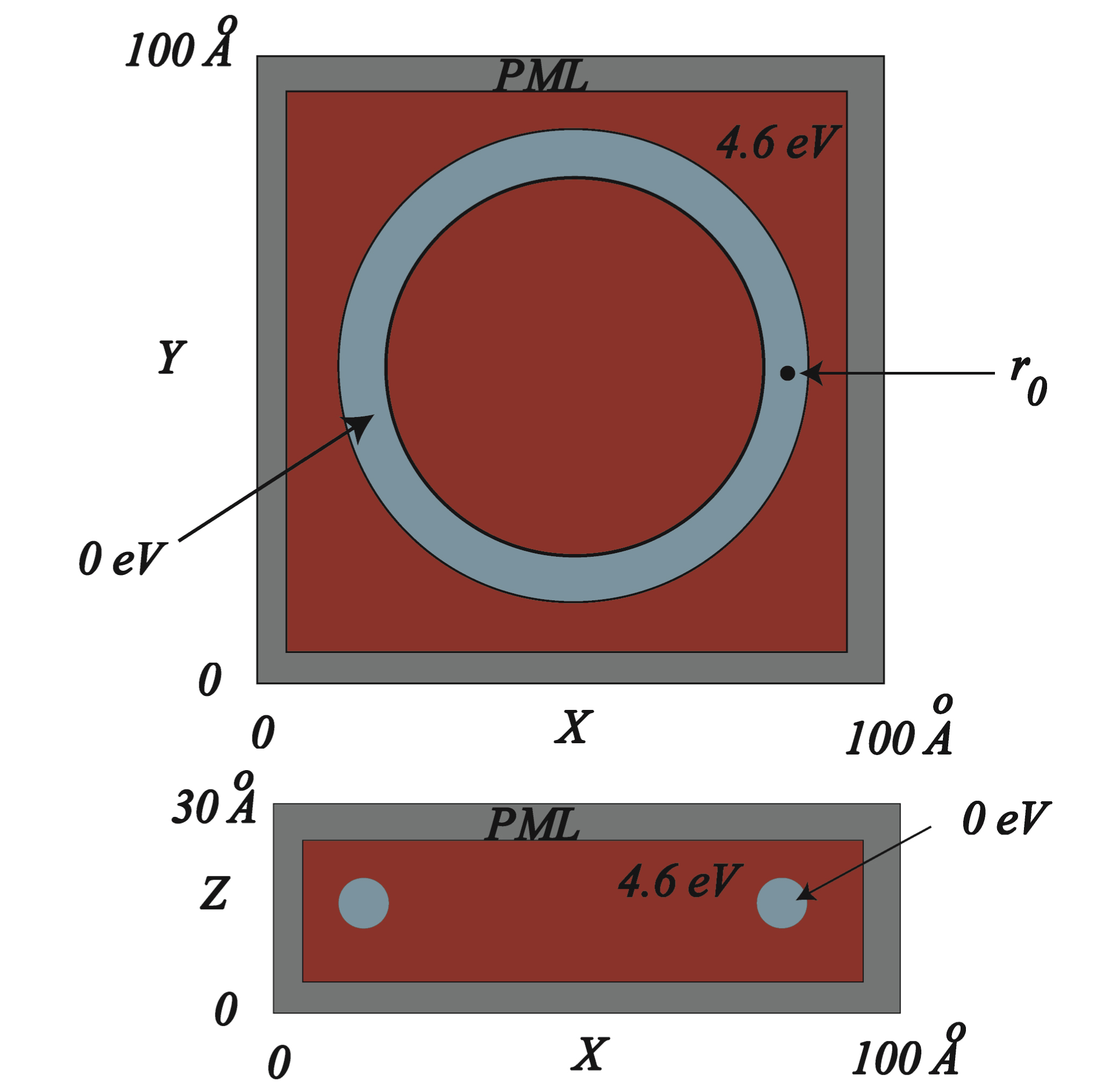
Figure 2: XY plane of the problem space containing the Torus...
XY plane of the problem space containing the Torus. The total problems space is 100 × 100 × 30 cells. The cells are one angstrom cubed.
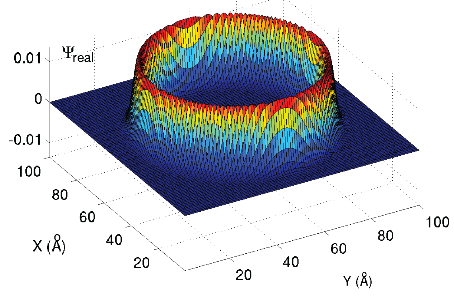
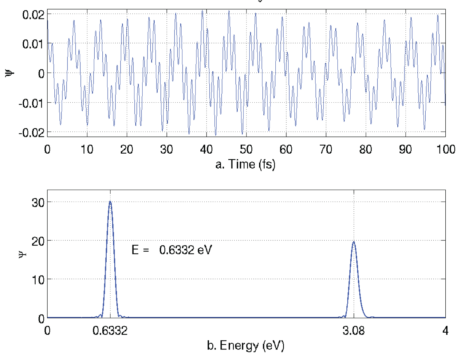
Figure 4: a) The time-domain plot of the wavefunction at the...
a) The time-domain plot of the wavefunction at the monitoring point ; b) The Fourier transform of the time domain data. Only the real part of the state function is shown.
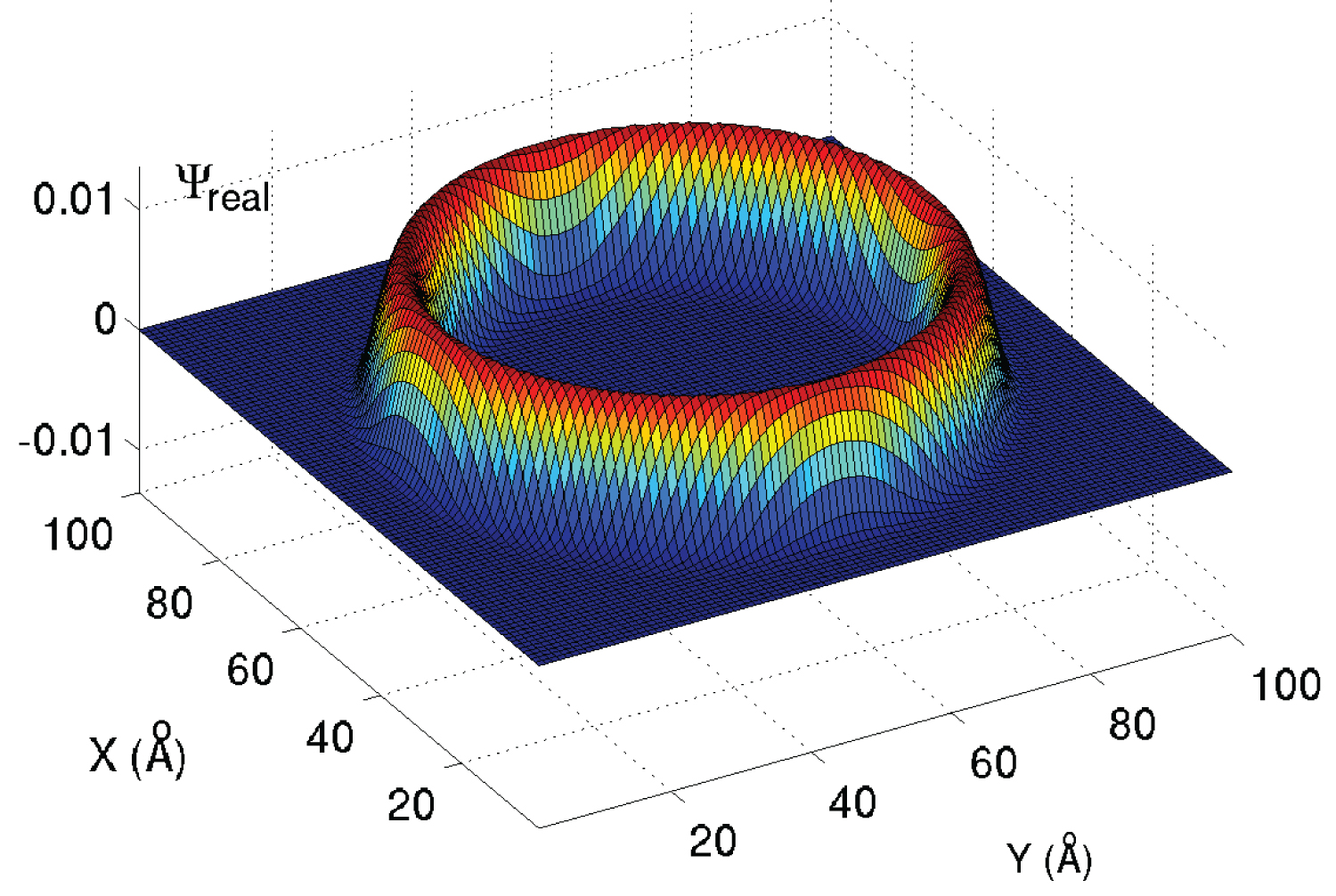
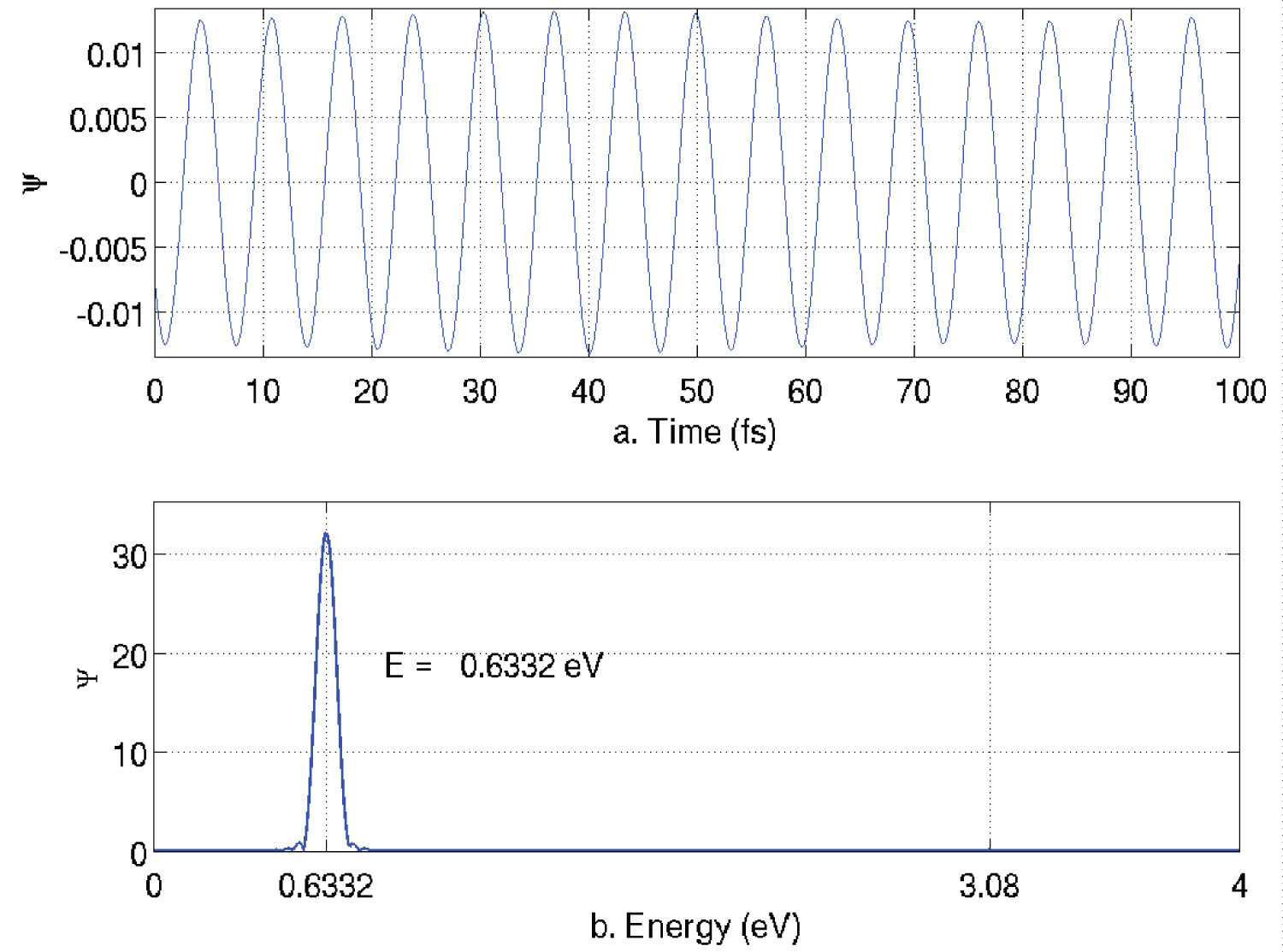
Figure 6: a) The time-domain plot of the wavefunction at the monitoring point...
a) The time-domain plot of the wavefunction at the monitoring point ; b) The Fourier transform of the time domain data.
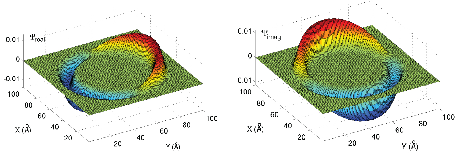
Figure 7: The real part (a) and the imaginary part (b) of the first...
The real part (a) and the imaginary part (b) of the first excited state in the torus.
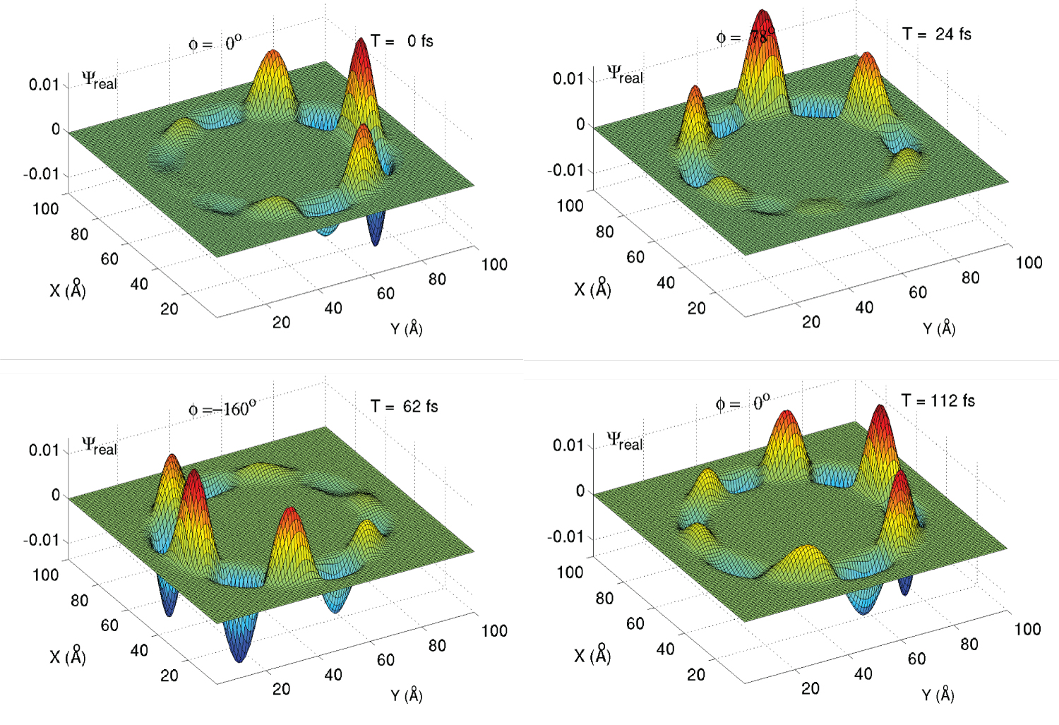
Figure 8: The sixth eigenstate confined within a radial Gaussian...
The sixth eigenstate confined within a radial Gaussian exponential. The waveform moves counterclockwise around the torus and returns to its original position after 111.6 fs.
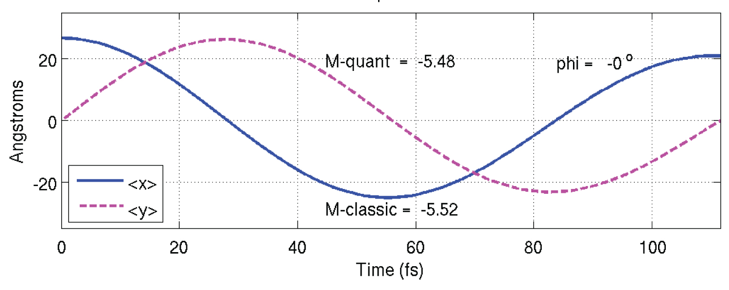
Figure 9: Plot of the expectation values in the X and Y directions...
Plot of the expectation values in the X and Y directions as a function of time. The units of M are .
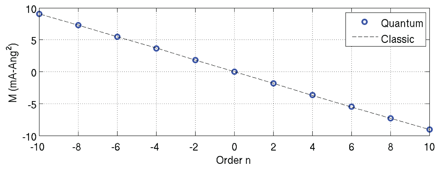
Figure 10: Comparison of the quantum expectation values and...
Comparison of the quantum expectation values and the classical values of the magnetic dipole moment for different orders of eigenstates.
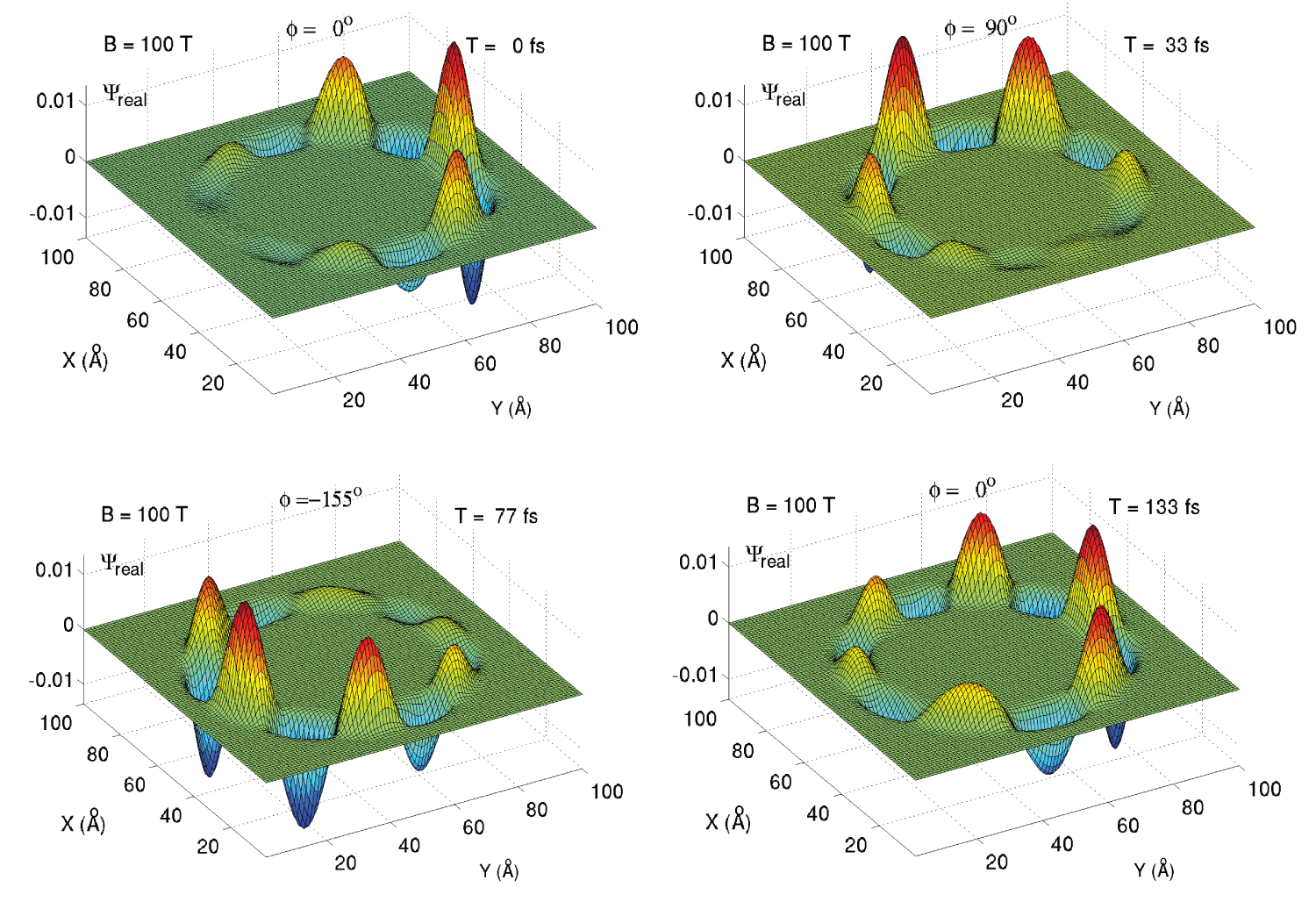
Figure 11: A repeat of the simulation illustrated in Figure 8, but...
A repeat of the simulation illustrated in Figure 8, but with magnetic field of -100 Tesla in the z direction.
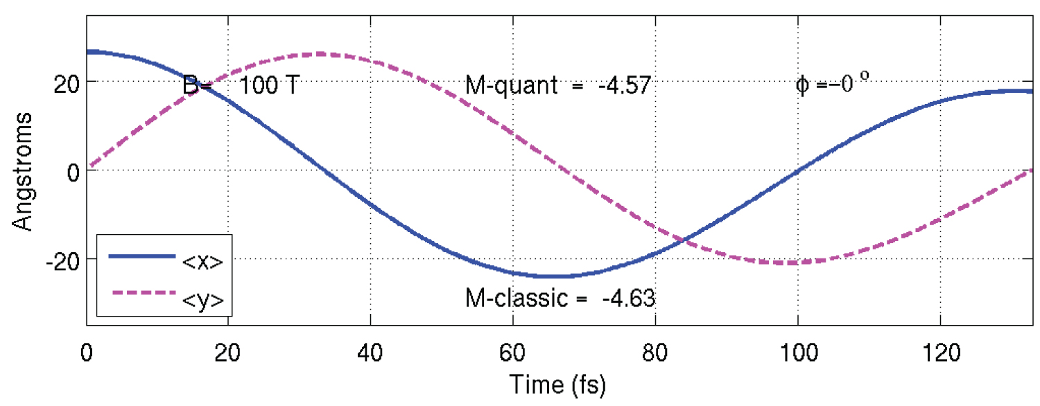
Figure 12: Plot of the expectation values in the X and Y directions...
Plot of the expectation values in the X and Y directions as a function of time, similar to Figure 9, but for the magnetic field of -100 Tesla in the z direction. The units of M are .
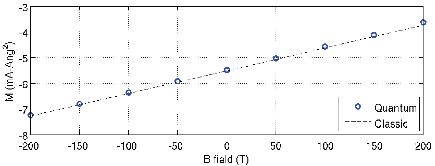
Figure 13: Comparison of the quantum expectation values and the...
Comparison of the quantum expectation values and the classical values of the magnetic dipole moment for various magnetic field strengths.
Tables
Table 1: The expectation value of the magnetic dipole moment operator (Eq. 10) for the torus of Figure 1, and the corresponding classical calculation (Eq. 11) as illustrated in Figure 10 for the various eigenfunctions of the torus.
Table 2: The expectation value of the magnetic dipole moment operator (Eq. 16) for the torus in Figure 1, and the corresponding classical calculation (Eq. 11) as a function of the applied magnetic field.
References
- DJ Brod, J Combe (2016) Passive CPHASE gate via cross-Kerr nonlinearities. Phys Rev Lett 117: 080502.
- DJ Brod, J Combes, J Gea-Banacloche (2016) Two photons co- and counterpropagating through N cross-Kerr sites. Phys Rev A 94: 02833.
- D Cotter, RJ Manning, KJ Blow, AD Ellis, AE Kelly, et al. (1999) Nonlinear optics for high-speed digital information processing. Science 286: 1523-1528.
- JE Heebner, RW Boyd (1999) Enhanced all-optical switching by use of a nonlinear fiber ring resonator. Opt Lett 24: 847-849.
- DM Sullivan (2013) Electromagnetic simulation using the FDTD method. (2nd edn), IEEE Press.
- DM Sullivan, DS Citrin (2001) Time-domain simulation of two electrons in a quantum dot. J Applied Physics 89: 3841-3846.
- DM Sullivan, DS Citrin (2003) Time domain simulation of quantum spin. J Applied Physics 94: 6518.
- Soriano, EA Navarro, PA Porti, V Such (2004) Analysis of the finite difference time domain technique to solve the Schrödinger equation for quantum devices. J Applied Physics 95: 8011-8018.
- GB Ren, JM Rorison (2004) Eigenvalue problem of the Schrödinger equations via the finite-difference time-domain method. Phys Rev E Stat Nonlin Soft Matter Phys 69: 036705.
- DM Sullivan, PM Wilson (2012) Time-domain determination of transmission in quantum nanostructures. J Applied Physics 121: 064325.
- DM Sullivan, S Mossman, M Kuzyk (2016) Time-domain simulation of three-dimensional quantum wires. PLoS One 11: e0153802.
- DM Sullivan, S Mossman, M Kuzyk (2016) Hybrid quantum systems for enhanced nonlinear optical susceptibilities. J Opt Soc Am B 33: E143-E149.
- JJ Sakurai (1994) Modern quantum mechanics. Addison Wesley.
- Messiah (2014) Quantum mechanics. Dover Publishing.
- MG Kuzyk (2000) Physical limits on electronic nonlinear molecular susceptibilities. Phys Rev Lett 85: 1218.
- MG Kuzyk, J Perez-Moreno, S Shafei (2013) Sum rules and scaling in nonlinear optics. Physics Reports 529: 297-398.
- Y Kivshar, A Miroshnichenko (2017) Meta-optics with Mie resonances. Optics and Photonics News 28: 24.
- MR Shcherbakov (2014) Enhanced third-harmonic generation in silicon nanoparticles driven by magnetic response. Nano Lett 14: 6488-6492
- DM Sullivan, DS Citrin (2002) Determination of the eigenfunctions of arbitrary nanostructures using time domain simulation. J Applied Physics 91: 3219-3226.
- DM Sullivan, DS Citrin (2005) Determining quantum eigenfunctions in three-dimensional nanoscale structures. J Applied Physics 97: 104305.
- DM Sullivan (2012) Quantum mechanics for electrical engineers. IEEE Press.
- W Dai, G Li , R Nassar, S Su (2005) On the stability of the FDTD method for solving a time-dependent Schrödinger Equation. Numerical Methods for Partial Differential Equations 21: 1140-1154.
- JP Berenger (1994) A perfectly matched layer for the absorption of electromagnetic waves. J Comput Phys 114: 185-200.
- C Zheng (2007) A perfectly matched layer approach to the nonlinear Schrödinger wave equations. J Compt Phys 227: 537-556.
- DJ Griffiths (1995) Introduction to quantum mechanics. Prentice-Hall.
- JD Jackson (1999) Classical electrodynamics. (3rd edn), Wiley.
- DK Cheng (1989) Field and wave electromagnetics. Addison-Wesly Publishing.
- AL Fetter, JD Walecka (2003) Theoretical Mechanics of particles and continua. Dover Publishing, New York.
Author Details
Jennifer Houle1, Dennis M Sullivan1*, Ethan Crowell2, Sean Mossman2 and Mark G Kuzyk2
1Department of Electrical and Computer Engineering, University of Idaho, USA
2Department of Physics and Astronomy, Washington State University, USA
Corresponding author
Dennis M Sullivan, Department of Electrical and Computer Engineering, University of Idaho, Moscow, Idaho, USA.
Accepted: March 08, 2018 | Published Online: March 10, 2018
Citation: Houle J, Sullivan DM, Crowell E, Mossman S, Kuzyk MG (2018) Three Dimensional Time Domain Simulation of the Quantum Magnetic Dipole. Int J Magnetics Electromagnetism 4:011.
Copyright: © 2018 Houle J, et al. This is an open-access article distributed under the terms of the Creative Commons Attribution License, which permits unrestricted use, distribution, and reproduction in any medium, provided the original author and source are credited.
Abstract
A method is presented to simulate the magnetic response of a quantum toroid for the purpose of optimizing the nonlinear characteristics of an induced magnetic dipole. This is a true three-dimensional simulation based on the direct implementation of the time-dependent Schrödinger equation. We demonstrate that the expectation value the quantum magnetic dipole operator returns results consistent with a classical electron in a loop under the influence of a magnetic field.
Keywords
Nonlinear optics, Induced magnetic dipole, Quantum simulation
Introduction
Nonlinear optics is a promising approach to the development of advanced computing [1,2] and communication technologies [3,4]. One of the challenges in the development of nonlinear optical systems is the search for materials with large nonlinear characteristics. Experimental approaches are both expensive and time-consuming. For this reason, computer simulation can play a significant role in the development of new nonlinear optical devices. The finite-difference time-domain (FDTD) method offers the possibility of true three-dimensional simulation of nanoscale nonlinear optical devices. The FDTD method is one of the most widely used in electromagnetic simulation [5] and has recently been applied to quantum simulation [6-10].
A previous paper describes the accuracy of the FDTD method in determining the eigenstates of quantum wires [11]. A subsequent paper describes the determination of the hyperpolarizability of quantum wires in close proximity to an electric dipole [12]. In this paper we describe the simulation of a magnetic dipole formulated as a quantum loop as well as the FDTD implementation of the quantum magnetic dipole operator. While electric dipoles are represented by the position operator, magnetic dipoles are represented by the angular moment operator [13,14]. Hence, the two moments are sensitive to different symmetries. Furthermore, it is of interest to see whether the magneto-optical response is bounded in the same manner as the electro-optical response [15,16]. In Mie theory, for example, the magnetic response can be larger than the electric response for certain systems [17,18].
In this paper we briefly review the FDTD implementation of the time-dependent Schrödinger equation. Specifically, we describe the simulation of a torus in three dimensions that will be used as the loop for a magnetic dipole. We then describe the use of signal processing techniques to determine the eigenenergies and eigenfunctions of a quantum torus [19-21]. Lastly, we describe the FDTD implementation of the magnetic dipole moment operator and a method based in classical electrodynamics to confirm the accuracy of the quantum operator.
The Finite-Difference Time-Domain Method
We begin by describing the FDTD implementation of the time-dependent Schrödinger equation [21], which is written in the following form
Where is the mass of an electron and is the potential seen by the electron.
We separate into real and imaginary components:
Inserting Eq. (2) into Eq. (1) leads to two coupled equations:
To code these equations, we take the finite-difference approximations in space and time that results in the following two coupled equations:
In Eq. (4) integer indices m, n, l representing the positions in a matrix have replaced the Cartesian coordinates x, y, z, respectively, in Eq. (3). Similarly, the time step k has replaced t. Once the cell size is chosen, the time step must also be chosen so the constants preceding the spatial Laplacian are small enough to maintain stability [22]. The alternate iteration of the real and imaginary Eq. (4a) and (4b) simulates the behavior of the evolution of in time. Details are available in the literature [6-8]. Figure 1 illustrates the quantum ring to be simulated. The ring is represented by a torus with a diameter of 70 angstroms. The tube of the torus has a diameter of 10 angstroms. The entire problem space is bordered by a perfectly matched layer (PML) [23,24] that can absorb outgoing waves that would otherwise interfere with the simulation. The implementation has been described in a previous paper [10] and will not be repeated here.
The problem space for the simulation is shown in Figure 2.
Determining the Eigenstates of the Torus
The FDTD method can be used to determine the eigenenergies and eigenstates of a potential that does not otherwise lend itself to an analytic solution [19,20]. Any quantum wavefunction of a given quantum system can be written in the following manner,
Where the are the eigenfunctions of the system and the are the corresponding eigenenergies. We can write the state variable in this fashion even if we do not know the eigenfunctions and eigenenergies.
The eigenenergies can be determined by monitoring the time-domain data at one point in the torus, say , and then taking the Fourier transform,
The last step results from the following property:
The above transform produces a series of delta functions in the frequency domain corresponding to the eigenenergies. Normally the initializing test function, in Eq. (5), is chosen to be a narrow pulse that will contain the eigenstates of interest. However, to search for the ground state of the torus illustrated in Figure 2, we found it more expedient to start with a test function that was radial symmetric within the torus, as shown in Figure 3. The FDTD simulation is started, and as time progresses the time-domain data is saved at the point in the torus. This is shown in Figure 4a. The Fourier transform of the time-domain function is shown in Figure 4b. Notice that the first peak in Figure 4a corresponds to the ground state energy of . The smaller component at 3.08 eV is likely due to the oscillation of the wavefunction against the walls of the tube.
To determine the corresponding ground state eigenfunction , we take the discrete Fourier transform (DFT) of the state variable at the frequency at every point in the problem space:
This results in the waveform shown in Figure 5. To check that this is truly an eigenfunction we can once again monitor the time variation of the ground state function as the FDTD simulation is run. The time-domain data is shown in Figure 6a, and the Fourier transform is shown in Figure 6b. Note that only the frequency component corresponding to the ground state energy results, indicating that the function in Figure 5 is indeed the ground state eigenfunction.
This process can be repeated for the higher order eigenstates, as shown in Figure 7. Figure 7a shows the real and imaginary parts of the wavefunction of the 1st eigenstate. The wavefunction will rotate in the counterclockwise direction in time, as will any of the positive eigenstates. Eigenstates corresponding to negative integers will rotate clockwise.
Calculation of the Magnetic Dipole Moment
The magnetic dipole operator when no B field is present is [25,26]
In this situation we need to include the spin component of the state. We write the total state as
Where χ describes the spin of the electron. The expectation value of the magnetic dipole moment is then
The spin term is quite simple and can be evaluated analytically. It introduces a constant offset of to the magnetic dipole moment.
With the spin contribution determined, the remainder of the paper will focus on the orbital contribution to the dipole moment, the pertinent operator now being
If the torus is in the XY plane, we need only be concerned with that component of M in the z direction
The partial derivatives are easily implemented in the FDTD formulation,
The constants ic and jc are the centers of the problem space in the x and y directions, respectively. Note that the derivatives are approximated over two cells.
To verify the accuracy of the quantum magnetic dipole moment calculation, we use the classical magnetic dipole moment for a current loop [27]:
Where is the radius of the loop. To simulate the current of an electron moving around the torus, we start with the n = 6 eigenstate, but confine the waveform with a radial Gaussian envelope around the z axis, as shown in Figure 8. As the waveform makes one complete circle around the loop, this represent a current of , where T is the time to make the circle.
To quantify the above simulation, the expectation values of the X and Y directions are determined at each step during the simulation, as shown in Figure 9. The angle of the particle can be determined by
This makes it easier to observe the length of time for one complete cycle.
One lap of the wavefunction around the torus, which corresponds to a classical current of one electron traveling the circumference of the torus, results in
Where , as shown in Figure 9 when the wavefunction has returned to its original position. Putting this in Eq. (11) gives
(We chose the units of to get manageable numbers.) The process was repeated for the eigenstates between -10 and 10. The results are shown in Table 1 and Figure 10. Clearly the agreement is very good.
Magnetic Dipole Moment in a Magnetic Field
When a magnetic field is present, the Hamiltonian becomes
If the magnetic field is restricted to the z direction, i.e.,
Then A becomes
And the Hamiltonian is
We have ignored the electric dipole interaction. The details of the implementation of Eq. (15) into FDTD have been described previously [6,7].
In the presence of a magnetic field in the z direction the angular momentum acquires another term [28], resulting in a modified magnetic dipole moment,
The implementation of the second half of Eq. (16) into FDTD is straight forward.
The simulations illustrated in Figure 11 and Figure 12 are repeated for magnetic fields between -200 Tesla and 200 Tesla at 50 Tesla intervals. The results are tabulated in Table 2, and are plotted in Figure 13. Clearly, the agreement is very good, but the error between the quantum and classical values increases for higher positive values of B, as seen in Table 2, where the errors between the quantum and the classical values only exceed one percent for .
Conclusion
We have shown that the FDTD method can be used to determine the characteristics of a nanoscale magnetic dipole. The accuracy of this method was established by comparing expectation values of the quantum magnetic dipole operator with the classical magnetic dipole moment.
The simulations described in this paper were done on an HP DL140 with eight cores, a high end workstation, and does not represent extraordinary computational resources. A typical simulation to determine the expectation of the magnetic dipole moment requires about 60 seconds.
Future projects include the use of the simulations described here to determine the first and second magnetic dipole hyperpolarizability as a function of the shape of the object, with the goal of finding the ideal geometry that maximizes the hyperpolarizability.
Acknowledgements
EC, SM, and MGK acknowledge the generous support of the National Science Foundation, Grant ECCS-1128076., and MGK acknowledges the Meyer Distinguished Professorship of the Sciences.