International Journal of Astronautics and Aeronautical Engineering
(ISSN: 2631-5009)
Volume 5, Issue 2
Original Article
DOI: 10.35840/2631-5009/7544

Article Formats
A Physical Aircraft Performance Model for Multi-Criteria Trajectory Optimization
Table of Content
Figures
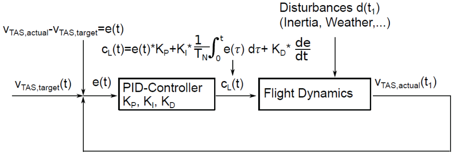
Figure 1: The control loop of COALA....
The control loop of COALA. The lift coefficient cL(t) is used as regulative variable to control true airspeed vTAS. The parameters KP, KI, KD and reset time TN depend on aircraft type, mass, and flight phase.
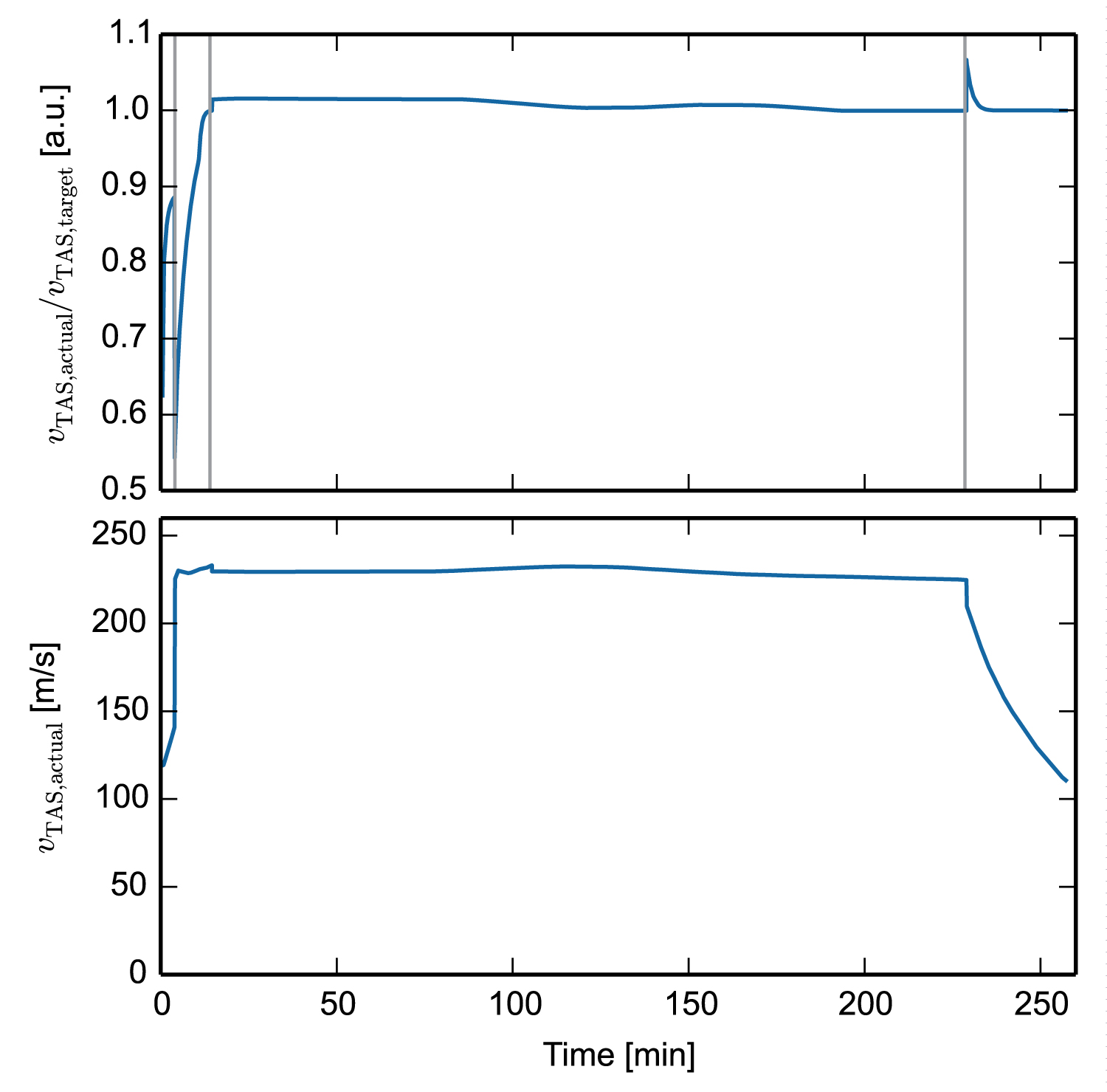
Figure 2: Top: The ratio of actual true airspeed.....
Top: The ratio of actual true airspeed vTAS,actual and target true airspeed vTAS,target as function of time demonstrates the efficacy of the PID controller and the inertia forces of a B777F aircraft which must not be neglected. Four flight phases are separated by vertical lines and indicate changes in target true airspeed vTAS,target which are achieved after a few time steps. Bottom: Absolute Values of the target true airspeed vTAS,target.
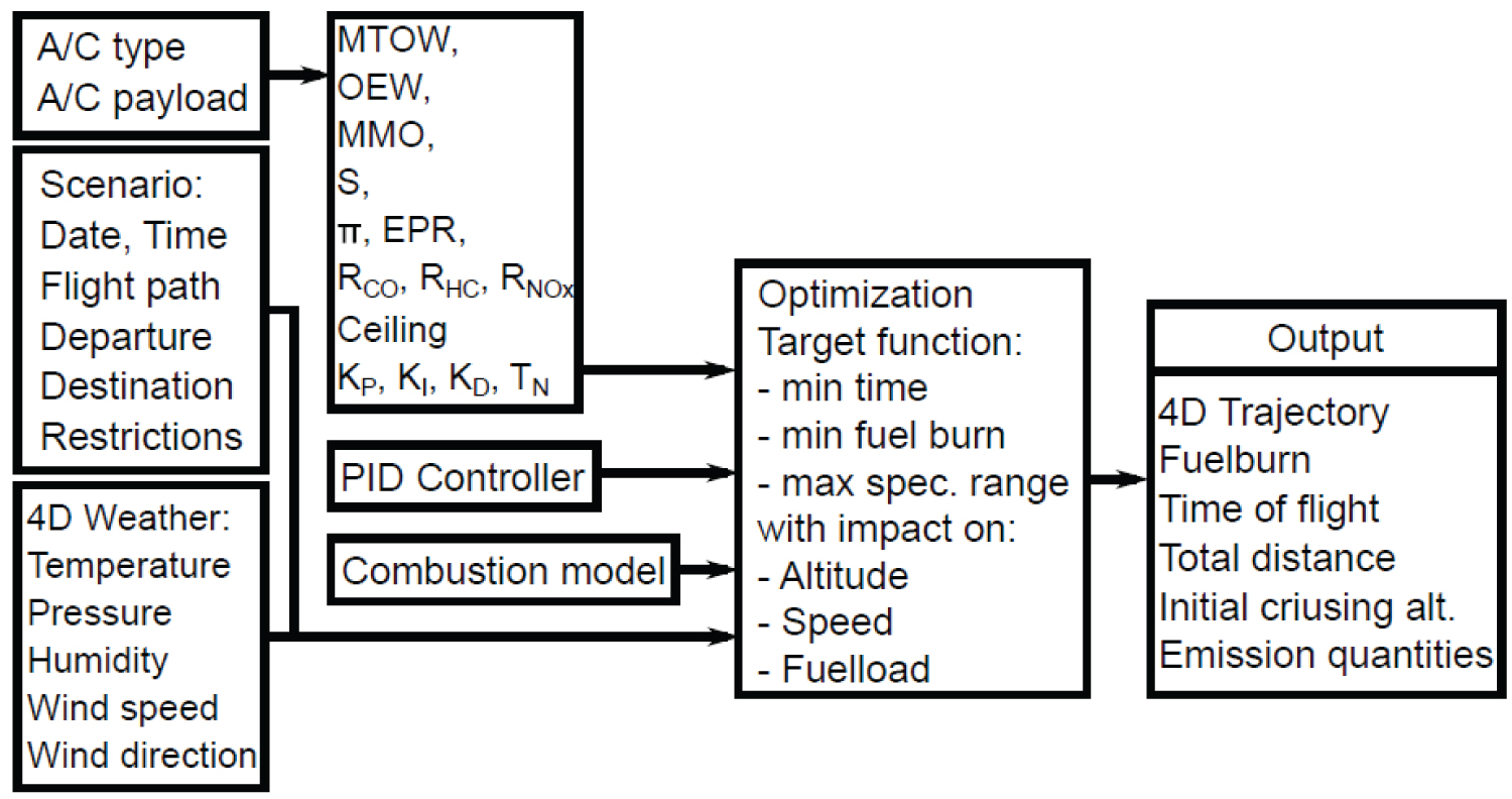
Figure 3: Structure, input variables, target....
Structure, input variables, target functions, output and sub models of the flight performance model COALA.
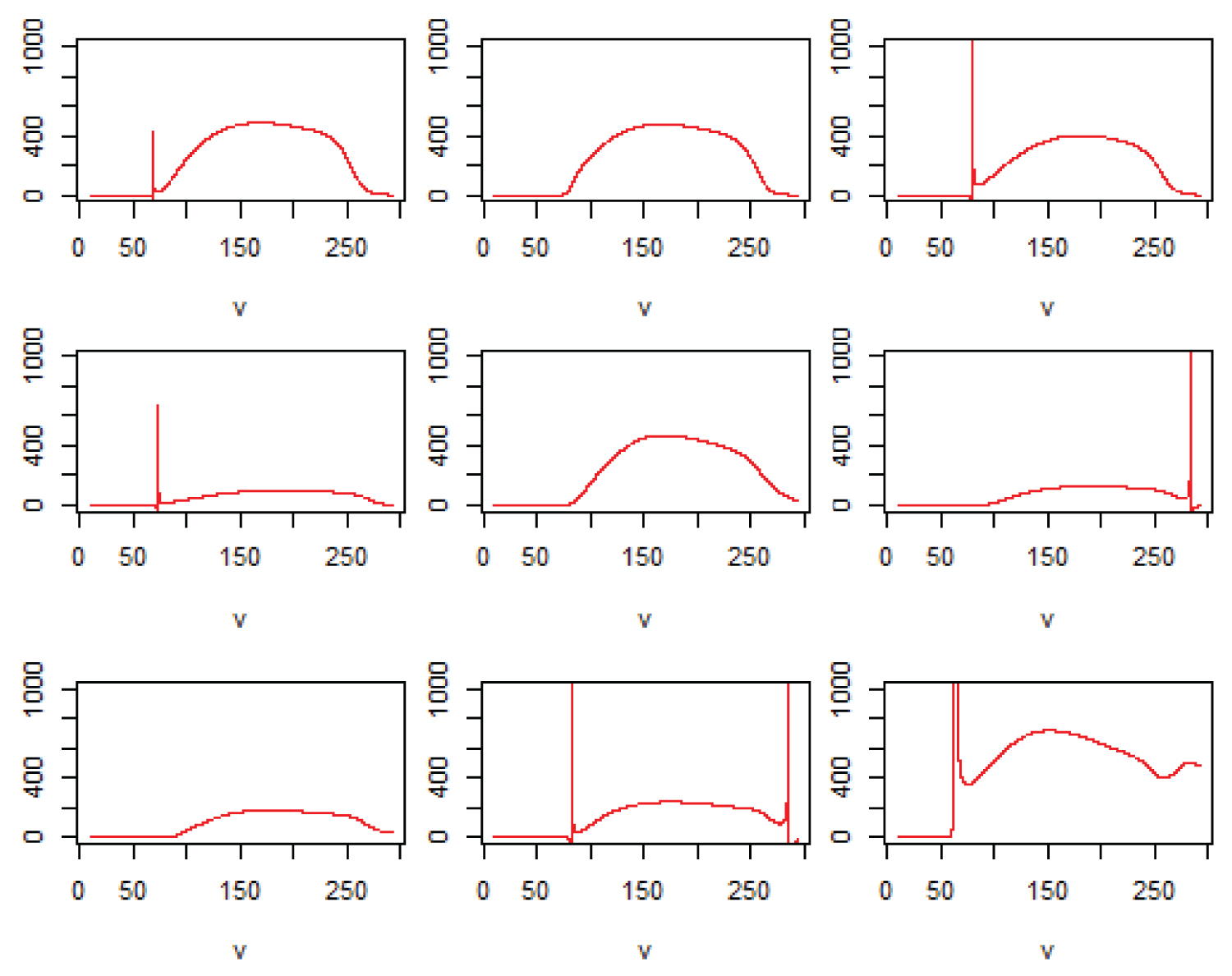
Figure 4: Specific range Rspec [mkg-1] as function....
Specific range Rspec [mkg-1] as function of true air speed vTAS [ms-1]. Each plot represents a different aircraft type (jet engine) with maximum take-off mass in 10'000 m altitude.
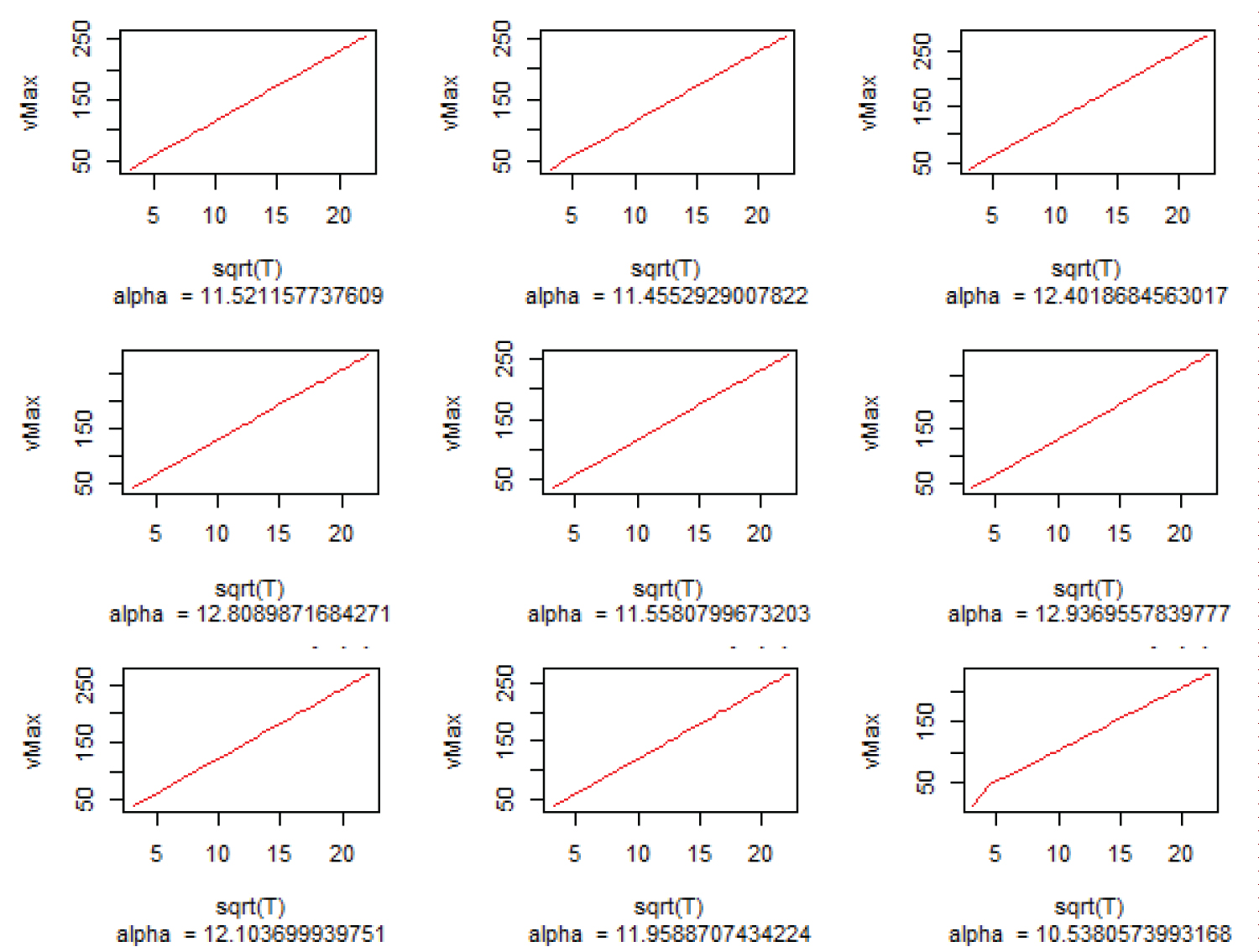
Figure 5: True air speed for a maximum specific....
True air speed for a maximum specific range as function of square root of atmospheric temperature vTAS(T) [ms-1]. Each plot represents a different aircraft type (jet engine) with maximum take off mass in 10'000 m altitude.
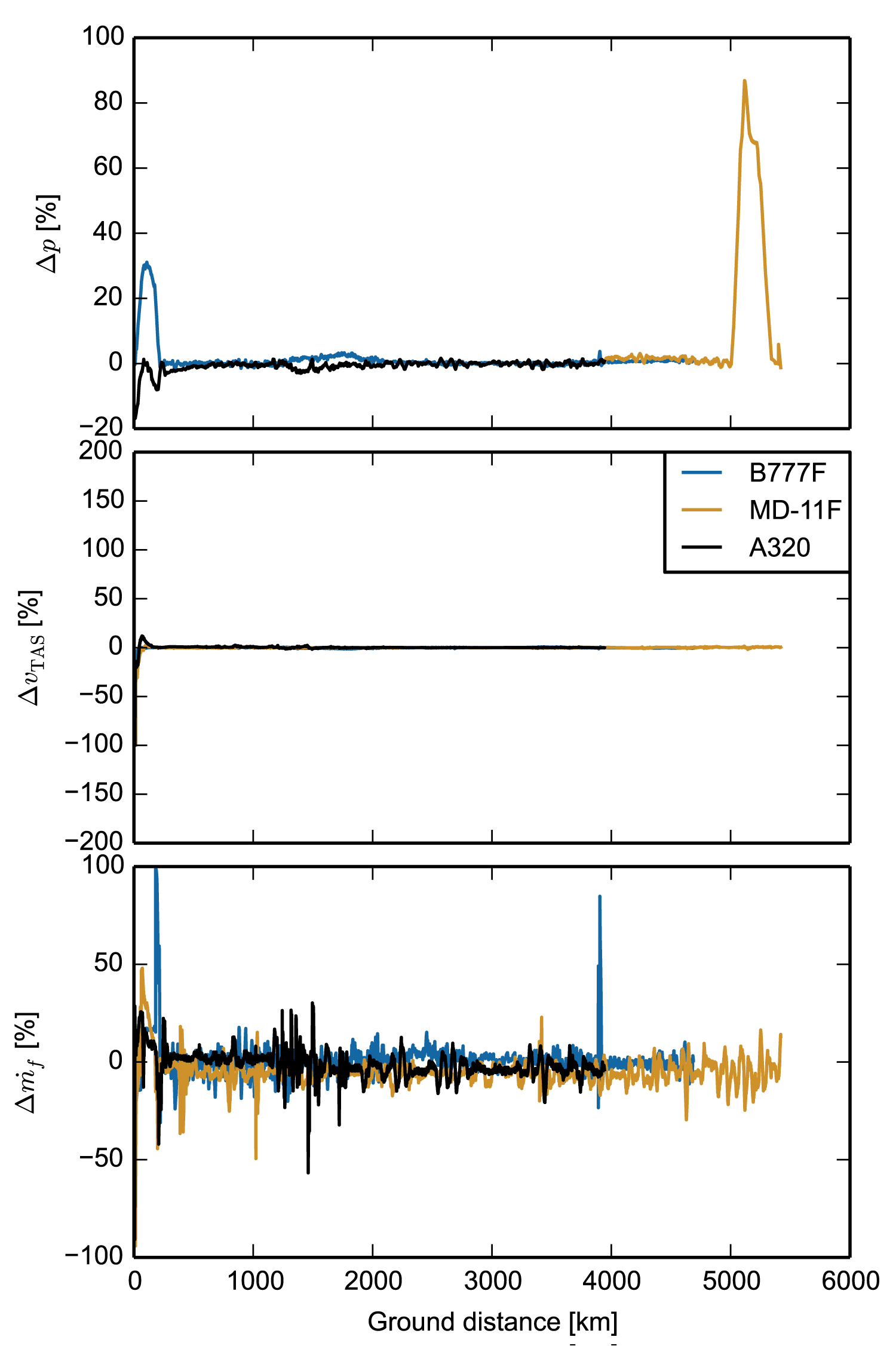
Figure 6: Real (black) and modeled (orange) pressure....
Real (black) and modeled (orange) pressure altitude (top), actual speed (middle) and fuel flow (bottom) of a B777F flight for validation purposes. COALA can follow given target values for speed and altitude and to reproduce the real fluctuations in fuel flow in the model.
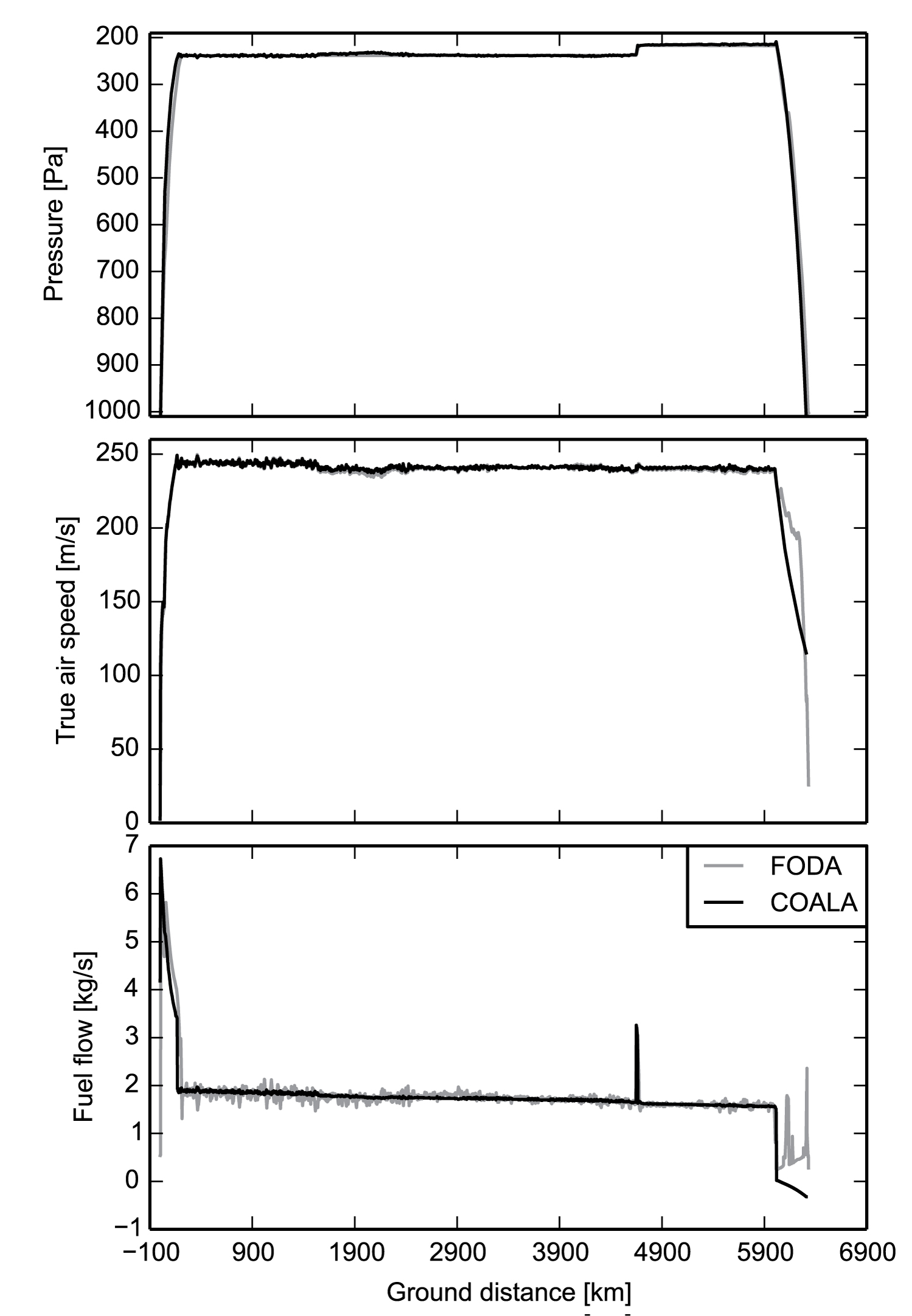
Figure 7: Small differences between real and modeled...
Small differences between real and modeled pressure (top), speed (middle), and fuel flow (bottom) of three single trajectories with different aircraft types indicate a realistic behavior of modeling aircraft type-specific performance and inertia with COALA.
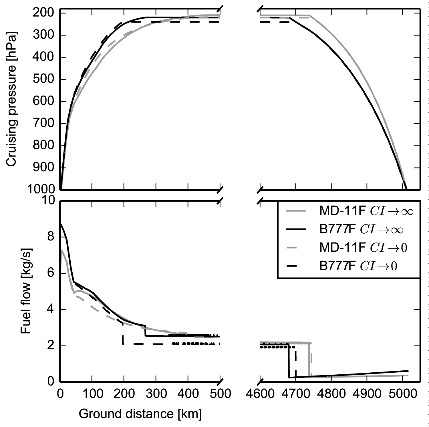
Figure 8: Comparison of pressure altitude (top)...
Comparison of pressure altitude (top) and fuel flow (bottom) of optimized B777F and MD-11F trajectories. MD-11F is characterized by a shallow climb profile (high drag polar) and high cruising altitudes (large amount of available thrust).

Figure 9: Top: Thrust of optimized trajectories....
Top: Thrust of optimized trajectories with respect to minimum flight time of the MD-11F (gray) and the B777F (black). Bottom: True air speed of the optimized trajectories of both aircraft. A low OEW and a large amount of available thrust causes higher MD-11F speeds, especially during climb and descent.
Tables
Table 1: Mean differences between real and modeled fuel flow [kg s-1], true air speed vTAS [m s-1] and pressure altitude p [Pa] for validation purposes of COALA.
Table 2: Optimized variables cruising pressure altitude pcruise and speed correction factor α with corresponding results of the time of flight and fuel burn for different objectives of optimization.
References
- J Rosenow, M Lindner, H Fricke (2017) Impact of climate costs on airline network and trajectory optimization: A parametric study. CEAS Aeronautical Journal 8: 371-384.
- SES Single european Sky (2004) Verordnung (eg) Nr. 549/2004 des europa¨ischen parlaments und des rates: zur Festlegung des rahmens fu¨r die schaffung eines einheitlichen europa¨ischen luftraums. Rahmenverordnung.
- (2015) SESAR Joint Undertaking, European atm master plan edition 2.
- A Abeloos, M von Paassem, M Mulder (2003) An abstraction hierarchy and functional model of airspace for airborne trajectory planning support. In Conference on human decision making and manual control, L University.
- S Forster, J Rosenow, M Lindner, H Fricke (2016) A toolchain for optimizing trajectories under real weather conditions and realistic flight performance. In Greener Aviation, Brussels, Belgium.
- (2012) User manual for the base of aircraft data (BADA) Family 4.
- (2004) User manual for the base of aircraft data (BADA) Revision 3.6. Eurocontrol, EEC Note No. 10/04.
- M Kaiser (2014) Optimierung von flugtrajektorien strahlgetriebener verkehrs-flugzeuge bei konkurrierenden sesar zielfunktionen mittels entwicklung eines hochprazisen flugleistungsmodells. Ph.D dissertation, Technische Universitat Dresden, Germany.
- M Kaiser, M Schultz, H Fricke (2012) Automated 4d descent path optimization using the enhanced trajectory prediction model (ejpm). In Proceedings of the International Conference on Research in Air Transportation (ICRAT).
- M Kaiser, J Rosenow, H Fricke, M Schultz (2012) Tradeoff between optimum altitude and contrail layer to ensure maximum ecological enroute performance using the enhanced trajectory prediction model (etpm). In: Proceedings of the 2nd International Conference on Application and Theory of Automation in Command and Control Systems (ATACCS), London.
- J Rosenow, M Kaiser, H Fricke (2012) Modeling contrail life cycles based on highly precise flight profile data of modern aircraft. In Proceedings of the International Conference on Research in Airport Transportation (ICRAT).
- M Kaiser, M Schultz, H Fricke (2011) Enhanced jet performance model. In: Proceedings of the 2nd International Conference on Application and Theory of Automation in Command and Control Systems (ATACCS).
- M Schultz, H Fricke, M Kaiser, T Kunze, J Lopez-Leone´s, et al. (2011) Universal trajectory synchronization for highly predictable arrivals. In SESAR Innovation Days (SID).
- M Soler, B Zou, M Hansen (2014) Flight trajectory design in the presence of contrails: Application of a mulitphase mixed-integer optimal control approach. Transportation Research Part C 48: 172-194.
- R Dalmau, X Prats (2015) Fuel and time savings by flying continuous cruise climbs: Estimating the benefit pools for maximum range operations. Transportation Research Part D: Transport and Environment 35: 62-71.
- J Rosenow, S Forster, H Fricke (2016) Continuous climb operations with minimum fuel burn. In Sixth SESAR Innovation days.
- B Sridhar, H Ng, N Chen (2011) Aircraft trajectory optimization and contrails avoidance in the presence of winds. Journal of Guidance, Control, and Dynamics 34: 1-13.
- RSF Patron, RM Botez, D Labour (2014) Flight trajectory optimization through genetic algorithms coupling vertical and lateral profiles. In ASME 2014 International Mechanical Engineering Congress & Exposition.
- A Murietta Mendoza, R Mihaela Botez (2014) Vertical navigation trajectory optimization algorithm for a commercial aircraft. In American Institute of Aeronautics and Astronautics 2014-3019.
- U Ringerz (2004) Aircraft trajectory optimization as a wireless internet appliacation. Journal of Aerospace Computing Information and Communication 1: 85-99.
- R Howe-Veenstra (2004) Commercial aircraft trajectory optimization and effciency of air traffc control procedures. Master's thesis, University of Minnesota.
- CR Hargraves, SW Paris (1987) Direct trajectory optimization using nonlinear programming and collocation. Journal of Guidance Control and Dynamics 10: 338-346.
- M Bittner, F Holzapfel, B Fleischmann, M Richter (2014) Optimization of atm scenarios considering overall and single costs. In 6th International Conference on Research in Air Transportation.
- C Göttlicher, M Gnoth, M Bittner, F Holzapfel (2016) Aircraft parameter estimation using optimal control methods. In AIAA Atmospheric Flight Mechanics Conference.
- D Wasiuka, M Lowenberga, D Shallcrossb (2015) An aircraft performance model implementation for the estimation of global and regional commercial aviation fuel burn and emissions. Transportation Research Part D: Transport and Environment 35: 142-159.
- JJ Lee, IA Waitz, BY Kim, GG Fleming, L Maurice, et al. (2007) System for assessing aviation's global emissions (sage), part 2: Uncertainty assessment. Transportation Research Part D: Transport and Environment 12: 381-395.
- P Morell, C Luc (2007) The environmental cost implication of hub-hub versus hub-bypass flight networks. Transportation Research Part D: Transport and Environment 12: 143-157.
- J Brueckner, R Girvin (2008) Airport noise regulation, airline service quality, and social welfare. Transportation Research Part B 42: 19-37.
- V Grewe, C Fromming, S Matthes, S Brinkop, M Ponater, et al. (2014) Aircraft routing with minimal climate impact: The react4c climate cost function modelling approach (v1.0). Geoscientific Model Development 7: 175-201.
- JA Lovegreen, JR Hansman (2011) Estimation of potential aircraft fuel burn reduction in cruise via speed and altitude optimization strategies. In MIT Inter- national Center for Air Transportation (ICAT), Cambridge.
- A Skowron, D Lee, RRD Leon (2015) Variation of radiative forcings and global warming potentials from regional nox emissions. Atmospheric Environment 104: 69-78.
- OA Søvde, S Matthes, A Skowron, D Iachetti, L Lim, et al. (2014) Aircraft emission mitigation by changing route altitude: A multimodel. Atmospheric Environment 95: 468-479.
- M Hrastovec, F Solina (2016) Prediction of aircraft performances based on data collected by air traffic control centers. Transportation Research Part C 73: 167-182.
- J Sun, J Ellerbroek, JM Hoekstra (2018) Aircraft initial mass estimation using bayesian inference method. Transportation Research Part C 90: 59-73.
- J Sun, J Ellerbroek, JM Hoekstra (2018) Wrap: An open-source kinematic aircraft performance model. Transportation Research Part C 98: 118-138.
- R Alligier, D Gianazza, N Durand (2013) Learning the aircraft mass and thrust to improve the ground-based trajectory prediction of climbing flights. Transportation Research Part C 36: 45-60.
- R Alligier, D Gianazza (2018) Learning aircraft operational factors to improve aircraft climb prediction: A large scale multi-airport study. Transportation Research Part C 96: 72-95.
- J Scheiderer (2008) Angewandte Flugleistung. Verlag Berlin Heidelberg, Springer.
- J Rosenow, S Forster, M Lindner, H Fricke (2018) Multicriteria-optimized trajectories impacting today's air traffic density, efficiency, and environmental compatibility. Journal of Air Transportation, 27.
- WJG Braunling (2009) Flugzeugtriebwerke. Verlag Berlin Heidelberg, Springer.
- DS Lee, G Pitari, V Grewe, K Gierens, JE Penner, et al. (2010) Transport impacts on atmosphere and climate: Aviation. Atmospheric Environment 44: 4678-4734.
- A Kugele, F Jelinek, R Gaffal (2005) Aircraft particulate matter emission estimation through all phases of flight. Eurocontrol.
- M Schaafer (2006) Methodologies for aviation emission calculation-A comparison of alternative approches towards 4d global inventories. Diploma Thesis.
- ICAO engine exhaust emissions databank, Doc 9646- AN/943.
- (2016) National Oceanic and Atmospheric Administration. Global data assimilation system (gdas).
- E Schmidt (1941) Die entstehung von eisnebel aus den auspuffgasen von flugmotoren. Schriften der Deutschen Akademie der Luftfahrtforschung, Verlag R. Oldenbourg, Munchen/Berlin 44: 1-15.
- H Appleman (1953) The formation of exhaust condensation trails by jet aircraft. Bulletin of the American Meteorological Society 34: 14-20.
- R Sussmann, KM Gierens (2001) Differences in early contrail evolution of two-engine versus four-engine aircraft: Lidar measurements and numerical simulations. Journal of Geophysical Research 106: 4899-4911.
- J Rosenow (2016) Optical properties of condenstation trails. Technische Universita t Dresden, Germany.
- J Rosenow, H Fricke (2019) Individual condensation trails in aircraft trajectory optimization. Sustainability 11: 21.
- (2018) Annex 14 - Aerodormes: Aerodromes Design and Operations. (8th edn), International Civil Aviation Organization, Tech Rep, 1.
- D Poles, A Nuic, V Mouillet (2010) Advanced aircraft performance modeling for atm: Analysis of bada model capabilities. In: 29th Digital Avionics Systems Conference.
- SK Clark, RN Dodge (1979) A handbook for the rolling resistance of pneumatic tires. Industrial development division.
- (2013) ICAO, Continuous climb operation (cco) manual.
- JD Anderson (1989) Introduction to flight. (3rd edn), McGraw-Hill, USA.
- (2010) Ratings and operating limitations for turbine engines. Federal Aviation Administration, Adivsory Circular.
- RP Brent (1973) An algorithm with guaranteed convergence for finding a zero of a function. Algorithms for minimization without derivatives.
- T Donchev, E Farkhi (1998) Stability and euler approximation of one-sided lips-chitz differential inclusions. SIAM Journal on Control and Optimization 36: 780-796.
- (2010) ICAO, Continuous descent operations (cdo) manual, 1.
- J Rosenow, D Strunck, H Fricke (2018) Trajectory optimization in daily operations. In International Conference on Research in Air Transportation (ICRAT).
- J Rosenow, D Strunck, H Fricke (2018) Free route airspaces in functional air space blocks. In Proceedings of the Seventh SESAR Innovation days, Austria.
- J Rosenow, H Fricke, M Schultz (2017) Air traffic simulation with 4d multi-criteria optimized trajectories. In Proceedings of the 2017 Winter Simulation Conference.
- J Rosenow, M Schultz (2018) Coupling of turnaround and trajectory optimization in an air traffic simulation. In Proceedings of the Winter Simulation Conference Gotenborg, Sweden.
- A Nuic, D Poles, V Mouillet (2010) Bada: An advanced aircraft performance model for present and futureatm systems. International Journal of Adaptive Control Signal Processing 24: 850-866.
- J Rosenow, H Fricke (2019) Impact of multi-criteria optimized trajectories on european airlineefficiency, safety and airspace demand. Journal of Air Transport Management 78: 133-143.
Author Details
Judith Rosenow*
Institute of Logistics and Aviation, Technische Universitat Dresden, Germany
Corresponding author
Judith Rosenow, Institute of Logistics and Aviation, Technische Universitat Dresden, Germany.
Accepted: December 21, 2020 | Published Online: December 23, 2020
Citation: Rosenow J (2020) A Physical Aircraft Performance Model for Multi-Criteria Trajectory Optimization. Int J Astronaut Aeronautical Eng 5:044.
Copyright: © 2020 Rosenow J. This is an open-access article distributed under the terms of the Creative Commons Attribution License, which permits unrestricted use, distribution, and reproduction in any medium, provided the original author and source are credited.
Abstract
In line with the objectives of making air transport safer, more efficient, and environmentally friendly through Trajectory Based Operations, a new aircraft performance model has been invented to calculate and optimize free route trajectories considering dynamic weather conditions and multi-criteria target functions. Therefore, the dynamic equation is solved analytically to consider continuous changes in speed and acceleration of this unsteady system. Therewith, the model is based solely on physical functions and calculates only physically possible trajectories. Sixteen aircraft and eighteen engine types are included, the aircraft specific behavior is modeled in detail, and emissions are quantified. Besides a validation, the derivation of several objective functions is shown. Successful trajectory optimization is demonstrated by a variation of the effective variables cruising altitude and target speed. Especially under real weather conditions, aerodynamically derived objective functions cannot be generalized for all aircraft types because in addition to strong wind effects individual aircraft dynamics mainly depend on the drag polar, the maximum Mach number, and the operating empty weight. The model can be used by all participants following Trajectory Based Operations to ensure a continuous recalculation and the exchange of the optimal trajectory in the flight planning phase and during the flight.
Keywords
Flight performance, Aircraft trajectory, Trajectory optimization, Trajectory based operations
Introduction
Motivation
The growing public awareness of the aviation impact on climate change forces aviation stakeholders more and more to search for climate-friendly solutions. Optimization potential has been found on several air traffic planning levels ranging from network design to fleet assignment and trajectory optimization [1]. Regardless of the planning level, flight performance modeling is necessary for a reliable optimization of the air traffic system because it is the smallest unit on which each air traffic optimization should be based. Since the foundation of the Single European Sky (SES) and the corresponding research program Single European Sky ATM Research (SESAR) in 1999, the reduction of the air traffic environmental impact is regulated by law [2] in Europe. In the SES Basic Regulation No 549/2014 [2], the objectives of SESAR are published aiming a warranty of sustainable development of the European air traffic sector. Besides the triplication of capacity, the increase of safety by a factor of 10, and the decrease of air traffic management costs by 50%, the environmental compatibility of each flight should be reduced by 10%.
With the SESAR Masterplan, the basic concept for the design of the future air traffic management (ATM) had been established by EUROCONTROL in 2012 to meet the SESAR targets by the introduction of an optimized flight trajectory [3]. Therein, the SESAR targets shall be carried out by "Moving from Airspace to 4D Trajectory Management". The first step towards this action is called the Trajectory Based Operations (TBO) and focusses on the deployment of airborne trajectories [3], which considers all constraints inflicted by the highly complex and dynamic environmental conditions [4]. Free routing is also targeted in this step, to enable optimized trajectories [3]. Free routes are freely planed routes between a defined entry point and a defined exit point constraint by published or unpublished waypoints [3]. These waypoints should originate from a multi-objective trajectory optimization considering the aircraft flight performance, its emissions, and external influences such as weather conditions, other air traffic, and restricted areas. Hence, a target function for each objective is necessary. For this purpose, the Compromised Aircraft performance model with Limited Accuracy (COALA) has been developed, which derives the target figure (i.e. the true airspeed vTAS) from objective functions and controls the vTAS with a proportional + integral + derivative controller. The 4D trajectory is achieved by the integration of the dynamic equation. COALA has been developed in the framework of the research project MEFUL, where an optimum between the reduction of the aviation environmental impact and the costs is estimated on different planning levels, ranging from the individual trajectory up to the network structure [1]. This optimization is realized by a simulation environment called Toolchain for Multicriteria Aircraft Trajectory Optimization (TOMATO) [5], which evaluates the simulated air traffic system by using several sub-models (COALA amongst others) and varies their input parameters until an optimum is reached.
State of the art
Flight performance can be modeled with different granularity depending on the intended use. However, for the sake of precise aircraft type-specific flight performance modeling, plenty of sensitive aerodynamical parameters and the boundary conditions due to atmospheric conditions have to be considered. In an International Standard Atmosphere (ISA), performance models are available for airlines, e.g. the commercial flight planning tool Lido/Flight 4D by Lufthansa Systems, with unknown precision and restricted availability for the community. Furthermore, the Base of Aircraft Data (BADA) by the European Organization for the Safety of Air Navigation (EUROCONTROL) [6,7] provides specific aircraft performance parameters and allows a performance modeling for a wide range of aircraft types. Some missing dependencies as compressibility effects in the calculation of the drag coefficient had been considered by Kaiser [8] resulting in more precise modeling of the aircraft performance, the Enhanced Jet Performance Model (EJPM). This model had been used and applied for several problems, for example for estimations of the energy share of kinetic and potential energy during continuous descent operations [9], for considerations of flight profiles without contrail formation [10], for the influence of aircraft performance properties on the contrail life cycle [11], for automated trajectories [9,12] and synchronization of automated arrivals [13]. However, EJPM cannot follow arbitrary target functions for speed and altitude intents. Furthermore, EJPM is neglecting acceleration forces and inertia forces which are crucial modeling the performance of aircraft with weights of 500 tons and more. Soler, et al. [14] modeled the flight performance with a 3-degree of freedom dynamic model depending on vTAS, heading, and flightpath angle in an ISA atmosphere, but with two-dimensional wind information from a national weather service. The model is restricted to conventional procedures. Therewith, only defined flight levels during cruise separated with 1000 feet are considered and an optimum cannot be detected. Dalmau, et al., [15] estimated the fuel benefits in the cruise phase only. Rosenow, et al. [16] already published the possible benefits in the climb phase. However, all these applications use a single target function (e.g. minimum fuel flow or minimum time) for the optimization, which seems insufficient with the conflictive SESAR targets in mind. Furthermore, these models depend on defined waypoints, which must be flown with the most efficient performance. Still, the difficulty is to define the optimized waypoints.
Multi-criteria optimization of trajectories in a horizontal plane has been done by Sridhar, et al. [17] under real weather conditions with a detailed horizontal flight performance modeling as a two-point boundary value problem. Patron, et al. [18] and Murietta Mendoza [19] used multi-level optimizations in 3D grid models. Anyhow, the flight performance is only approximated by a performance database, where fuel burn and the distance traveled is calculated depending on Mach number (or Indicated Air Speed (IAS)), gross weight, temperature deviation of the ISA standard atmosphere, and altitude. This approach only considers the reduction of fuel consumption or time of flight. Both Ringerz [20] and Howe-Veenstra [21] developed smooth optimized trajectories following constant IAS or constant Mach number and a constant altitude at cruise with a single, but variable target function considering a temperature deviation of the ISA standard atmosphere. Hargraves [22], Bittner [23] and Gottlicher [24] optimized trajectories as an optimal control problem, which is able to consider conflictive target functions and real weather conditions. The discrete input parameters are approximated by analytically solvable functions. From this follows, that only a restricted number of parameters can be considered and sometimes the errors done by the approximation seem too high. Furthermore, the flight performance is modeled in a very simple way. Interesting findings on the global impact of aviation on climate change have been made by Wasiuka, et al. by determining fuel burn and emissions with a flight performance model, which is however not suited for optimization [25]. Often, noise emissions are focused in aircraft trajectory optimization and air transport assessment, because, noise emissions are already implemented in airport charges. For example, Lee, et al. [26], Morell, et al. [27] and Brueckner, et al. [28] considered airport noise regulations beside airline service and social welfare in a global analysis. The research project REACT4C of the German national aeronautics and space research center (DLR) published interesting findings regarding ecological trajectory optimization [29-31] and [32]. However, all these approaches cannot be generalized due to the major impact of the assumed atmospheric conditions.
Missing aircraft-specific parameters in flight performance modeling can partly be derived from flight history data (ADS-B). Although this rarely achieves the precision of BADA, it is independent of commercially available data sets and can be published more easily. Particularly successful in this respect were Hrastovec, et al. [33], Sun, et al. [34,35], and Alligier, et al. [36,37].
Flight Performance Methodology
Principle model functions
With the 4D flight performance model COALA, the impact of aircraft type-specific aerodynamics and the important influence of three-dimensional weather information both affecting an optimized trajectory in the actual operational flight is obtained. COALA considers plenty of sensitive parameters. On the one hand, the flight performance is described by true airspeed vTAS, thrust FT [N], fuel flow [kg s-1], forces of acceleration ax [m s-2] and az [m s-2], time of flight t [s], and emission quantities [kg s-1]. On the other hand, aircraft type specific aerodynamical parameters A like wing area S [m2], maximum Mach number MMO, the number of engines, aircraft weights, and the drag polar depending on flap handle position and Mach number are considered.
For each time step, COALA continuously calculates target values of vTAS, altitude z, and flight path angle γ. vTAS,target, ztarget and γtarget are used as controlled variables in an aircraft type specific proportional plus integral plus derivative controller (PID controller). The lift coefficient is the regulating variable in this PID controller, ensuring flight performance and aerodynamic limits (e.g. MMO, stall speed, and maximum lift coefficient). Real weather conditions induce constant changes in aircraft speed and acceleration and transform the aircraft performance modeling into an unsteady system. Due to this non-negligible fact, forces of acceleration permanently act on the aircraft. The optimization target of COALA's controller is to minimize this acceleration in all flight phases. The dynamic equations [38] in the horizontal plane
and in the vertical plane
are integrated to derive the true airspeed and the air distance flown in each time step. FL denotes lift [N], FD drag, FG the aircraft weight [N], m the aircraft mass [kg] and ax, az the acceleration [m s-2] in the horizontal and vertical plane, respectively. Lift
and drag
depend on the lift coefficient cL [a.u.] and drag coefficient cD [a.u.] and air density ρ [kg m-3]. From equations 1 to 4 follows the definition of the flight path angle γ [rad]
Except from the take-off phase, the lift coefficient cL is the regulative variable in the PID controller and vTAS is the controlled variable (see Figure 1). Each time step, the difference between actual true air speed vTAS,actual and target true air speed vTAS,target denotes the error value e(t)
e(t) = vTAS,actual(t - 1) - vTAS,target (t). (6)
Each time step, the lift coefficient cL(t) is calculated by
The function of the PID controller is depicted in Figure 1. The parameters KP, KI, KD, and TN are determined for each aircraft type and flight phase and sometimes depend on the aircraft mass. For an A320 aircraft, KP, KI, KD and TN are in the order of magnitude of 10-1, 10-6, 10-1 and 10-1, respectively. The quality of the parameters strongly influences the ability of COALA to realistically represent the forces acting on the aircraft.
By regulating cL with the controller and by assuming that no flaps are extended during flight, the lift coefficient regulates the angle of attack of the aircraft. This procedure also takes place in the actual operation.
The drag coefficient cD is a function of Mach number, flap position and lift coefficient. Unless the aircraft is not included, BADA revision 4.1 [6] provides the function for cD. Otherwise, the BADA model 3.6 [7] is used. True airspeed vTAS,actual and air distance AD are calculated by integrating ax and az with a discrete time resolution of ∆t = 1s. Ground speed and ground distance are calculated after a wind correction. For the correction of the crosswind component, the aircraft heading is corrected by wind correction angle which is estimated from the crosswind component of the previous time step. The target function for vTAS can be derived from given Mach numbers, from target functions (one is explained in Section 3.3.1) and from given ground speeds (derived from a given cost index). Additionally, each target value can be adjusted by a speed correction factor α (see Section 3.2). In the case of three-dimensional weather information, COALA requires a lateral flight path, given in geographical coordinates (longitude and latitude) at an adequate number of sampling points (see Section 2.2.2). Between these supporting points, the flight path is calculated by linear interpolation. Spiraling is considered with speed depending minimum curve radius rmin [m] and load factor n [a.u.]. Usually, the simulation environment TOMATO (Toolchain for Multi-criteria Trajectory Optimization) [5,39] is used for the optimization of the lateral flight path. In the case of one-dimensional weather information, the great circle distance between start and destination is sufficient.
For estimating fuel flow and emission quantities, a jet engine-specific combustion model following [40-42] and [43] is implemented. The initial volume flow sucked in by the engine fan V0 is determined iteratively with the objective that the result must converge to a constant value. Thereby, the approximation of the fuel flow by BADA functions as a target value. The products of complete combustion CO2, H2O, SO2 and H2SO4 are estimated proportional to the fuel flow according to Lee, et al. [41]. The products of incomplete combustion NOx, CO and HC are calculated by using the state of the art Boeing-2 Fuel Flow method as described by Schafer [43]. For the quantification of the soot emissions, combustion inlet temperature T3 and pressure p3 are calculated following Kugele, et al. [42].
COALA can model five different flight phases with different parameters for the PID controller and different target functions for vTAS, altitude, and γ. The comparison of target values for speed, path angle, and altitude with the corresponding state variables allows the proof of both the PID controller and the derived target functions (compare Figure 2).
Triggers allow us to combine several flight phases to a complete flight. The triggers and the specifications of each flight phase are described in Sections 3.1 to 3.4. An overview over the structure, input variables, objective functions, output, and sub-models of COALA is provided by Figure 3.
Input variables
Input variables are considering a set of aircraft type-specific flight performance parameters A, scenario-specific variables, and environmental variables.
Aircraft type-specific parameters A: The following jet engine driven aircraft types are covered from Airbus (A310, A319, A320, A321, A330, A350, A380), Boeing (B737, B747, B767, B787, B777), McDon-nell Douglas (MD-11), Bombardier (CRJ900) and Embraer (E170, E190). For each aircraft type, operating empty weight OEW [kg], maximum take-off weight MTOW [kg], maximum payload, maximum fuel load, maximum Mach number MMO [a.u.], wing area S [m2] and service ceiling [m] as maximum cruising altitude are stored in a database. Additionally, for calculating the emission quantities the jet engine-specific combustion model uses engine pressure ratio EPR [a.u.], bypass ratio Π [a.u.] and the reference emission quantities for carbon monoxides CO [g kg-1], unburned hydrocar bons HC [g kg-1], nitric oxides NOx [g kg-1], and soot number [a.u.] depending on a thrust-specific fuel consumption [kg s-1] from the ICAO Aircraft Engine Emissions Databank provided by EASA [44].
Scenario-specific variables: Departure and destination, scheduled time of arrival, date and time of departure, number of passengers, payload [kg], fuel mass [kg], and optional thrust derate and the flight path as list of coordinates of longitude [°] and latitude [°] or as list of waypoint names define scenario-specific input variables. Additionally, specifications of the target functions for optimization for each flight phase are required besides end triggers (altitudes, speeds, distance, or time of flight) of each flight phase. Furthermore, the option of a dynamic optimization (with dynamic input variables, such as weather data) can be activated.
Environmental variables: The date and time of departure are used to identify the best matching weather data file. The weather data with the variable spatial resolution are taken from GRIB2 (GRIdded Binary) data, provided by the National Weather Service NOAA [45]. Weather data between the given data points are achieved by linear interpolation. The following weather data are used: Temperature T [K], air density ρ [kg m-3], pressure p [Pa], wind speed for Eastward u and Northward v directions and relative humidity rH [a.u.]. Alternatively, COALA can deal with one-dimensional weather information in form of a Standard Atmosphere (e.g. ISA).
Output variables
COALA calculates the vertical trajectory of each flight phase with fixed time steps ∆t = 1s and generates a 4D trajectory for both the aerodynamic and the Earth-fixed coordinate system. At least the aircraft position, altitude, actual flight path angle and target flight path angle, track, actual vTAS and target vTAS, actual lift coefficient and target lift coefficient, air distance and ground distance, ground speed, and the remaining fuel mass are provided for each second.
Additionally, engine specific data of fuel flow and engine emissions of carbon dioxide CO2, water vapor H2O, nitric oxides NOx, soot, sulfur oxides SO2, sulfuric acid H2SO4, carbon monoxides CO and unburned hydrocarbons HC are provided for each second. Furthermore, the formation of contrail formation is estimated according to the Schmidt-Appleman criterion [46,47] and the existence of ice-supersaturated regions [48]. The application is shown in [49,50].
Flight Phases
Take-off
For take-off, az = 0 and ax is calculated by
Where μ (FG-FL) = Fx [N] describes the frictional force on the landing gear and FG-FL = Fz [N] the bearing strength on the landing gear.
For take-off, the lift coefficient cL is linearly approximated as function of flap position and angle of attack AOA.
For take-off, the lift coefficient cL is linearly approximated as function of flap position and angle of attack AOA. During low speeds (or low weights), crosswind affects the aircraft controllability and stresses the tire side force capability. For that reason, aircraft manufacturers and airlines define maximum crosswind components depending on the size of the vertical stabilizer compared to the area of the whole aircraft exposed to the wind. This maximum crosswind component usually amounts to 16 m s-1 for a B737-800 or 20 m s-1 for a B777. Additionally, airports can limit the maximum crosswind component to ensure a safe take-off and landing performance. For example, London City Airport limits the crosswind component to 16 m s-1. Crosswind is measured at ten meters altitude. Since these limits denote very small values, the crosswind component is neglected in COALA during take-off. The required take-off thrust FT depends on aircraft mass, take-off distance available, atmospheric temperature, and altitude [51]. Following [52] the maximum take-off thrust
MTO = 1.33 MCL, (9)
can be described as function of maximum climb thrust MCL [N] depending on altitude for BADA3.6 aircraft types, whereas BADA4.1 provides coefficients for MTO. In order to consider a derated thrust, FT is linearly interpolated between MTO for aircraft with maximum take-off weight MTOW and MCL, if the aircraft weight corresponds with OEW. A thrust derate depending on outside air temperature is not implemented yet. It will be considered for future research.
The rolling friction coefficient is configurable between The default rolling friction coefficient represents a mean value for aircraft on a wet runway [38] or tires of large trucks on asphalt [53].
The acceleration along the runway 8 is integrated assuming vTAS(t = 0) = 0
vTAS = ax t (10)
The aircraft accelerates until the rotation speed vrotate is reached. In this case, the lift force FL exceeds the weight force FG by 30%. assuming a lift coefficient cL(AOA = 10°), gear down and a typical aircraft type-specific flap position (e.g. 1+F for A320):
For take-off, the lift coefficient as function of AOA and flap position β [-]
depends on aircraft type specific coefficients mcL,AOA, mcL,0 and mcL,β, which are developed from a comparative literature research. For example, for the B777F, the following coefficients are used: mcL,AOA = 5.5, mcL,0 = 0.29 and mcL,β = 1.4.
As soon as vrotate is reached, the aircraft is rotated with a rotation rate of 1° per second until AOA = 10°.
Climb
As soon as rotation is finished, the climb is operated as continuous climb operation without any step [54]. During the climb phase, two phases are distinguished [1]. A maximum climb angle γ is used as target function below 10000 ft altitude. The corresponding true airspeed vTAS,target is derived from an extremum determination of Equations 1 and 2 which are combined to
Here, a is the acceleration projected on the flight path, cD is a function of lift coefficient and speed [6,7] and the lift coefficient is controlled in order to achieve vTAS,target. This speed induces the geometrically steepest climb [55] for quickly reaching an altitude of 10000 ft with a minimum investment in kinetic energy.
Following FAA's Advisory Circular AC No:33.7-1 [56], the aircraft may be operated with maximum take-off thrust for a maximum of five minutes. For this reason, the thrust is reduced linearly to MCL during the fourth and fifth minutes after launch. MCL is used for the remaining climb phase.
Above 10000 ft the target function for vTAS,target maximizes the climb rate ω
in Equation 13 in order to utilize a maximum gain in altitude per time unit [55].
The cost index CI
of this climb, flight converges to CI → 0, because the aircraft invests the maximum amount of the energy in potential energy until the optimum cruising altitude is reached. Once at cruising altitude, the flight is more fuel-efficient due to lower air density. In Equation 15, Ct and Cf denote the cost of time and the cost of fuel , respectively. To achieve climb gradients different from the steepest possible ones, an increase of vTAS,target is configurable. This results in a shallower climb angle γ and in a reduced time of flight (CI > 0), because more energy is converted into kinetic energy. This configuration is called speed adjustment by a variable factor α.
Cruise
Already during the climb, the optimal cruising altitude is continuously calculated. Per default, altitude and true airspeed for a maximum specific range are numerically calculated. The optimum altitude depends on vTAS,max, which is a function of altitude z, and Brent's Method [57] is used for finding altitude and speed for each time step (find details in Section 3.3.1). Therewith, a flight with a continuous cruise climb can be modeled.
Furthermore, desired cruising pressure altitudes can be configured. As soon as the aspired cruising pressure altitude pcruise [Pa] or geometric altitude hcruise [m] is reached, COALA uses dummy flights to calculate the optimum time to initiate the cruise phase. The goal of the optimization is a smooth phase transition into cruise flight with new parameters KP, KI, KD, and TN for the controller.
Even during the cruise, especially under real weather conditions, the aircraft performance model COALA describes an unsteady system, because speed and acceleration are still constantly changing. Hence, Equation 13 has to be solved for every time step.
During cruise, vTAS,target is still controlled with a PID controller. Per default, the target value of vTAS,target is gained from a target function, which is the maximum of the specific range Rspec [m kg-1] calculated with Equation 13
Each time step the required thrust FT is estimated from Equation 13, for vTAS,target assuming a stationary equilibrium (i.e. FL = FG). Therewith, additionally to the controlled angle of attack, the target true airspeed is controlled by the thrust setting. Furthermore, FT will be increased, if the target pressure altitude was not reached in the last time step. The maximum cruise thrust is set to MCRZ = 0.95 MCL for BADA3.6 aircraft [52]. For BADA4.1 aircraft types, MCRZ is calculated depending on altitude and speed [6].
As described in Section 3.2, vTAS,target can be manipulated by a factor α, resulting in a trajectory with CI > 0. Furthermore, a desired calibrated airspeed vCAS, ground speed vGS or Mach number can be transformed in a corresponding vTAS,target. Therewith, conventional flight procedures can be modeled.
In the case vTAS is controlled, vTAS (Rspec,max) should be derived from Equation 16. Since fuel flow is a function of vTAS, the estimation of vTAS (Rspec,max) depends on the mathematical formulation of fuel flow depending on vTAS, aircraft mass m [kg], altitude z [m] and temperature T [K]. In BADA 4 [6] vTAS (Rspec,max) cannot be estimated analytically. Additionally, for some aircraft types Equation 16 shows inhomogeneities in the operational speed interval (see Figure 4). For that reason, beside a numerical extremum estimation, a numerical approximation is applied.
Numerical approximation of a speed for a maximum specific range: Following the BADA 4 manual, Equation 16 depends on:
Where Λ covers a set of functions depending on aircraft mass m [kg], atmospheric pressure p [Pa] and atmospheric temperature T [K] and A covers flight performance specific parameters, such as the aircraft wing area S [m2] and the lift to drag polar depending on speed and altitude. Hence, Rspec = f (vTAS, p, m, T, A). Fuel flow is formulated as
Where is a rational number, N is a very large integer (order of half a thousand) and is a relative integer. Note, , N and depend on the parameters of Rspec = f (vTAS, p, m, T, A). Furthermore, is only defined on an aircraft type-specific interval: [a; b]. Figure 4 gives an impression of Rspec as function of vTAS for different aircraft types with maximum take-off weight (MTOW) in 10000 m altitude. Figure 4 and Equation 17 show, that the function is not continuous for some aircraft types (e.g. top left, top right, middle left, middle right...). It is assumed, that this discontinuity has no physical value, it is the result of the empirical parameterizations to best fit the general function in Equation 17. Thereby, artificial zeros appear in some functions. Without those discontinuities, Equation 17 seems to be a physically plausible and continuous function with compact support. It covers the increased fuel required for very low and very fast speeds and a maximum in a physically reliable range of speed (i.e. between 150 and 200 ms-1).
Because the function is discontinuous, it is non-Lipschitzian [58]. However, a comprehensible impact of atmospheric temperature T has been identified. For a constant mass, a linear dependence on can be derived from the influence of the speed of sound Figure 5). as a very strict upper boundary of the maximum estimation (compare Figure 5).
Figure 5 shows a linear function of with the aircraft type-specific gradient α:
α can be approximated as function of altitude z [m], aircraft mass m [kg] and aircraft type-specific parameters A by
In Equation 20,
describes the finite value of α for aircraft with maximum take-off weight depending on altitude.
describes the finite value of α for aircraft with OEW. Finally,
determines the slope of a linear part of α(m) for small values of m depending on altitude.
The aircraft type-specific variables in Equation 20 are stored in the aircraft database. The errors of the fitted tanh function are in the range of 10-1 m s-1. With this method, a true airspeed for a maximum gain in vTAS per unit rate of fuel flow is approximated.
In case a Standard Atmosphere is assumed, the optimum pressure altitude p(Rspec) can be calculated by replacing atmospheric parameters in Equation 13 (and functional relationships therein) by functions describing the Standard Atmosphere. Under real weather conditions, p(Rspec) differs for every time step dt. In this case, a pressure altitude is either expected as an input parameter or derived from a target function. For example, the dependence of vTAS,max on altitude z is used to calculate the optimum altitude using Brent's Method [57] for finding altitude and speed for a maximum specific range.
Descent
With dummy descent flights, the top of descent (TOD) is iteratively calculated during the cruise, considering the actual aircraft weight, vTAS, and the corresponding rate of descent. The descent is initiated, as soon as the aircraft reaches the aspired distance or geographical coordinate. A continuous descent operation [59] down to the final approach fix in 10000 ft altitude is modeled. Due to strict safety regulations, approach, flare, and landing are not implemented yet, because these phases do not pose a potential for optimization. During descent, the engines operate in idle mode. Idle thrust coefficients and fuel flow are taken from BADA [6,7]. The target value for vTAS is continuously derived from an extremum determination of the lift to drag ratio E [a.u.]
Again, vTAS is controlled by a PID controller and regulated with the lift coefficient cL. The resulting angle of descent is calculated following Equation 5 and the descent rate ω is estimated with the use of Equation 23.
Validation
COALA had been validated with 40 sets of Flight Operational Data (FODA) of three aircraft types (Boeing B777F, McDonnell Douglas MD-11F, and Airbus A320). For each time step (every two seconds), true airspeed and altitude provided by real flight FODA data had been used as target functions for COALA (see Figure 1). Modeled fuel flow, actual speed, and actual altitude have been compared with the real data (see example flight in Figure 6). For each aircraft type, differences between reality and model have been averaged in Table 1.
Over 13 randomly chosen MD-11 flights, the average difference in pressure between COALA and the real flights is 464 Pa over the entire flight and 130 Pa only taking into account the cruising phase. The speed was mapped with a mean difference of 0.9 m s-1 and fuel flow had been calculated with an accuracy of 0.05 kg s-1 (more details in Table 1). Although the mean differences often are very small, sometimes the standard deviation is quite significant. For example, over 22 flights of Boeing B777F the mean difference between COALA and the real flight in pressure is about 228 Pa, but the standard deviation 431 Pa. These results include 3 obvious outliers without whose the mean is about 97 Pa and the standard deviation 268 Pa. Due to unknown weather conditions during the real flights, the ISA Standard Atmosphere had been used for modeling those flights with COALA. Thereby, significant differences between ground speed and ground distance may occur, resulting in inaccuracies of the model. Considering single flights, differences between real and modeled fuel flow, speed, and pressure are sufficiently small and fluctuate around Zero (shown in Figure 7).
Table 1 demonstrates that COALA can model the dynamics and forces acting on the behavior of a real aircraft. Using a target speed and a target altitude as input variables, COALA derives the correct ratio of investment in potential and kinetic energy. The PID controller adjusts the angle of attack based on the given ratio so that a correct gain in altitude and speed is modeled. Due to the high temporal resolution, realistic fluctuations in speed and fuel flow are depicted in Figure 6.
Results
COALA has been used for various applications ranging from single trajectories with precise weather information [16,60,61] to traffic flows [39,62,63]. Aircraft type-specific characteristics and prospects of COALA become clear when comparing two different air freighter, Boeing B777F and McDonnell Douglas MD-11F (with two GE-90 110B1L engines and three CF680C2D1F engines, respectively) along a flight path between Frankfurt, Germany (EDDF) and Dubai, United Arab Emirates (OMDB) with weather data from 2016, February, 2nd, 12 a.m. (Figure 8, Figure 9, and Table 2). Table 3 gives the aircraft characteristics. The payload of both aircraft is set to 70000 kg.
When optimizing trajectories of both aircraft, a different behavior especially during climb and descent emphasizes the capability of COALA to deal with different aircraft behavior (see also Figure 8). Here, the optimization functions where minimum fuel burn, minimum time of flight, and minimum emissions. Therefore, the cruising altitude and the proportional speed adjustment α act as variables by always respecting aircraft type-specific aerodynamical flight envelopes (i.e. boundaries of cL, MMO, service ceiling, MTO and MCL). In Figure 8 vertical profiles of optimized aircraft trajectories with minimum time (solid) and minimum fuel (dashed) are shown. The trajectories follow an optimized lateral path considering wind speed and wind direction at cruising pressure altitude.
Aircraft specific differences
The optimized cruising altitudes are realistic, considering the take-off weight of TOWB777F = 285150 kg and service ceiling (Table 3). The steep climb angle of the B777F results from the higher thrust and the lower drag polar (compare Figure 8), compared to the MD-11F. Furthermore, the lower drag polar of the B777F causes a shallower descent angle (Figure 8).
Both the high OEW and the low drag polar provoke low target values of vTAS (see Figure 9) and a steeper climb angle for the B777F. The increased gain in altitude (i.e. a larger angle of attack) of the B777F results in both time and fuel savings, compared to the MD-11F. The target function of the maximum climb rate (Equation 23) yields higher values at the expense of vTAS. For both aircraft, the target value of vTAS is limited to MMO = 0.87. This speed restriction is more relevant for the MD-11F, than for the B777F, because of the thrust surplus.
Note, the mentioned differences may additionally result from different BADA models used with different functional relationships. Especially, drag polar and fuel flow, which depends on altitude and Mach number in BADA 4.1 (as shown in Equation 17), but on thrust in BADA 3.6 [64]. The maximum cruise thrust is proportional to the maxim climb thrust in BADA 3.6, but depend on altitude and speed in BADA 4.1 [6].
Trajectory optimization
Decreasing air density with altitude causes a decrease in FD with altitude as long as the aircraft can generate enough lift without vTAS exceeding MMO. From this follows, that aerodynamically optimized true airspeed, flight path angle, and altitude can be derived from Equations 13, 16 and 24. However, under real weather conditions, the aerodynamic optimum pressure altitude need not be the global optimum, because altitude dependent wind manipulates the ground speed and therewith the time of flight. The change in wind direction and wind speed with altitude is hard to predict. With the variables, pcruise and α, the optimum can be searched iteratively. The variable α (varied 0.9 α 1.12) results in a change in vTAS and γ. A target speed vTAS exceeding the speed for maximum specific range causes a shallower climb gradient because more energy is converted into kinetic energy. Hence, the time of flight is reduced and fuel burn is increased. An increased vTAS in the target function by the speed correction factor α does not lead to higher cruising altitudes for the B777F, although the aircraft has already burned more fuel by reaching the top of the climb. The results of the trajectory optimization are shown in Table 2. As expected, the minimum time of flight is reached for α > 1, at the value of α that corresponds to the MMO during the cruise and at relatively high cruising altitudes. In general, fuel burn and vTAS are smaller for the B777F resulting in a long time of flight. Pressure altitude and vTAS of these optimized trajectories are shown in Figure 8 and Figure 9.
Conclusion and Outlook
The aircraft performance model COALA can calculate and optimize physically possible 4D trajectories. The equation of motion is solved analytically. The model differs from other aircraft performance models in the consideration of the forces of acceleration and inertia each time step by a PID controller, which controls the true airspeed and uses the lift coefficient as a regulative variable. The parameters of the controller are aircraft type specific. Therewith, COALA is based solely on physical functions, except for the drag polars, which are approximated using the BADA model. That's why COALA contains the "limited accuracy" in its name. COALA can calculate and optimize trajectories for several aircraft types. This paper demonstrates that aircraft type-specific behavior can be modeled in detail.
For trajectory optimization, the cruising altitude and the speed correction factor have been identified as effective variables to additionally consider the influence of weather conditions. The developed target function for vTAS (e.g. for a maximum climb rate or a maximum specific range Rspec) cannot be generalized for all aircraft types, especially not under real weather conditions. Individual aircraft type-specific target functions mainly depend on the drag polar, maximum Mach number, and operating empty weight.
In this paper, the results of the included emission model and the possibilities of multi-criteria trajectory optimization have not been shown, because the priority was given to the characteristics of COALA and its ability to simulate aircraft type-specific differences in the flight performance and trajectory optimization. In cooperation with the simulation environment TOMATO [1,5,39] COALA has already been used for multi-criteria trajectory optimization where emissions were included in the target function. Therefore, performance indicators have been transformed into costs. However, these cost functions would have exceeded the scope of this paper.
For trajectory optimization, COALA uses target functions for speed and altitude and allows mass-specific changes in speed and altitude. Today, operations consist of operational constraints. To meet these constraints, restrictions for both objective functions have been applied following the current navaid structure or airway structure [39,65]. To perform in Trajectory Based Operations, COALA has been successfully applied to fixed waypoints at fixed time steps as well [60,61]. The implementation of these constraints is necessary for trajectory prediction for all stakeholders, but always induces a deviation from the optimum.
Following the SESAR path to the Target Operational Concept, enhanced en-route airspace structures, multiple route options, modular temporary airspace structures, and reserved areas are the first step towards a flexible sectorisation management to enable Trajectory Based Operations [3]. Hence, freely optimized trajectories are expected to be a standard in a future operational environment.
Exactly for this application, COALA was developed to calculate an optimal trajectory anytime and anywhere and to share it with all stakeholders.
Acknowledgments
The author would like to thank Thomas Rosenow for programming support, Stanley Forster and Thomas Zeh for improving COALA.