
International Journal of Astronautics and Aeronautical Engineering
(ISSN: 2631-5009)
Volume 9, Issue 1
Research Article
DOI: 10.35840/2631-5009/7566
Analysis of the Influence of Two Turbulence Models on the Numerical Results of a Computational Fluid Dynamics Simulation for the NACA 0012 Airfoil Profile at Low Speeds
Augusto Henrique de Miranda Lima* and Luiz Joaquim Cardoso Rocha
Table of Content
Figures

Figure 1: Geometry of the NACA 0012...
Geometry of the NACA 0012 Airfoil - Due to its symmetry (non-cambered profile), it is widely adopted in academic research and experimental tests.
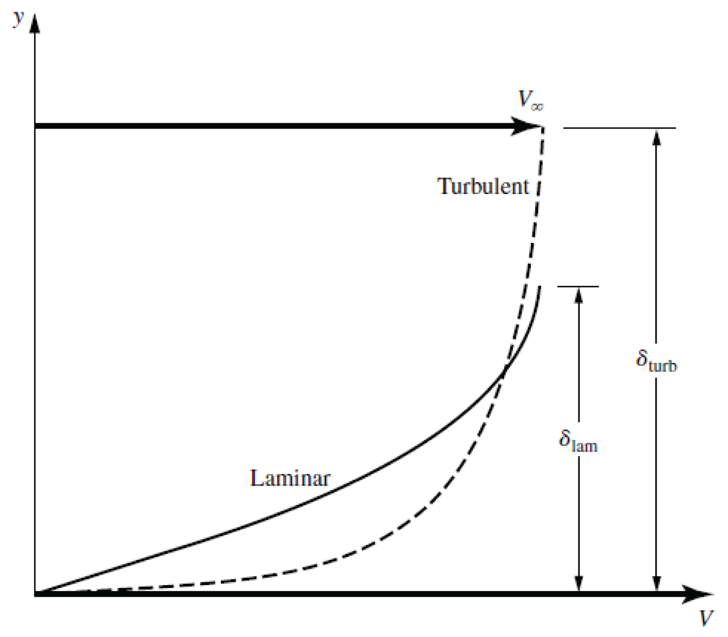
Figure 2: Velocity profiles for laminar....
Velocity profiles for laminar and turbulent boundary layers - Having higher velocity on the surface is detrimental in terms of drag, but regarding the detachment of the boundary layer, this excess velocity is desirable.
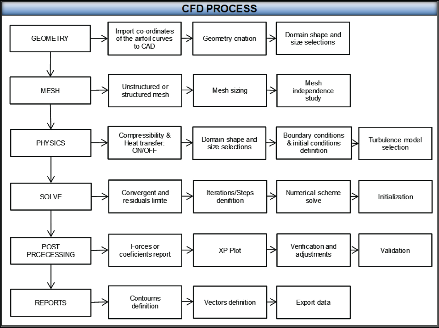
Figure 3: CFD process - CFD techniques....
CFD process - CFD techniques involve a set of mathematical models solved through numerical methods, utilizing computational processing, to obtain information about thermal exchanges, fluid flow, and other processes.
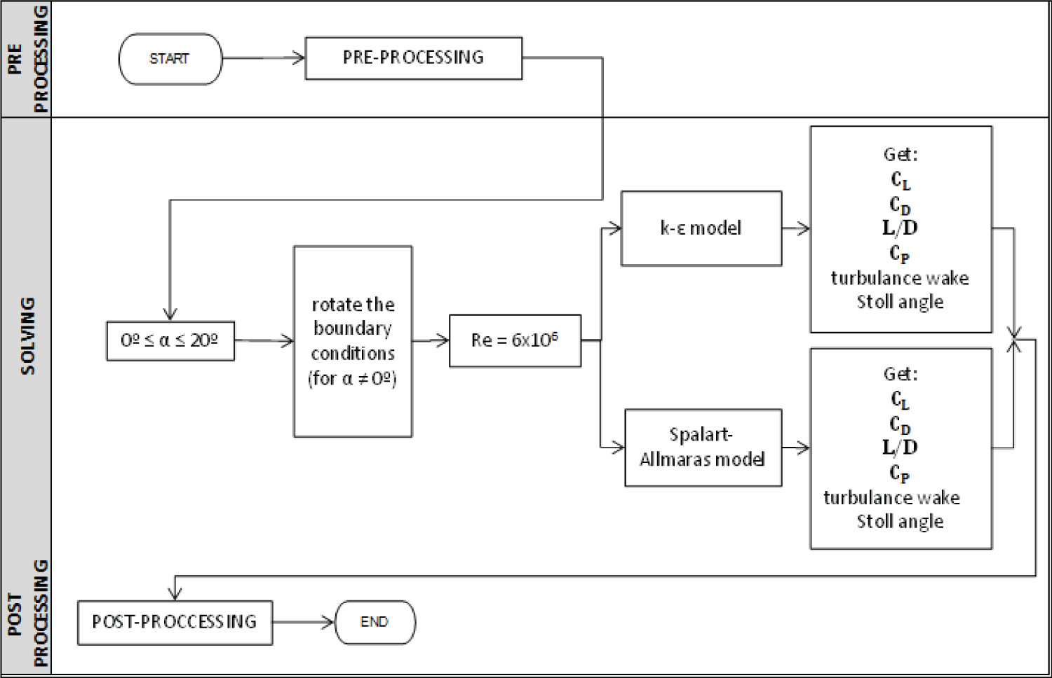
Figure 4: Procedures for conducting....
Procedures for conducting simulations - In total, disregarding the mesh independence test, 42 different scenarios were simulated to meet the objectives of this research.
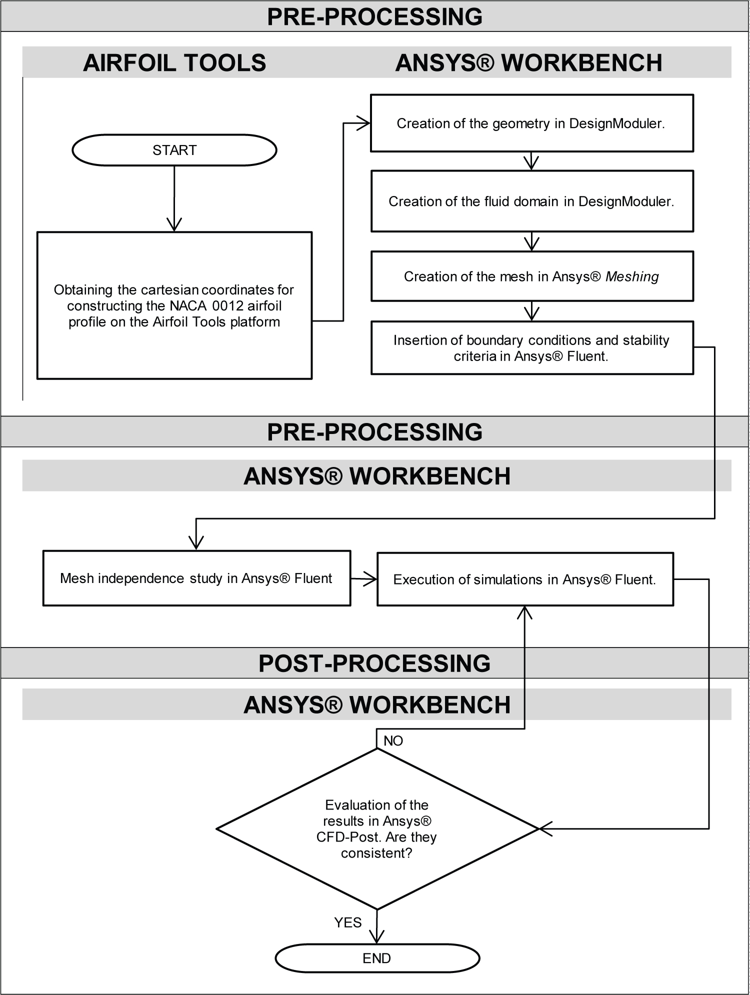
Figure 5: Execution methodology -....
Execution methodology - All numerical analysis was performed using the ANSYS® software package, specifically the Academic Student version 2022 R1.
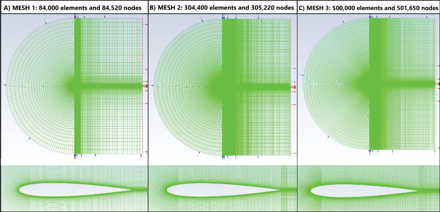
Figure 6: Mesh generated in Ansys....
Mesh generated in Ansys® Meshing - The obtained result was a structured mesh with quadrilateral elements.
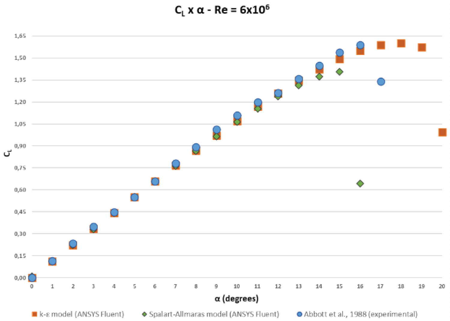
Figure 7: Comparative results for...
Comparative results for - It was identified that the is achieved at α = 15° and 18°, respectively, in the Spalart-Allmaras and k-ε realizable models. This was characterized as the stall angle of the profile.
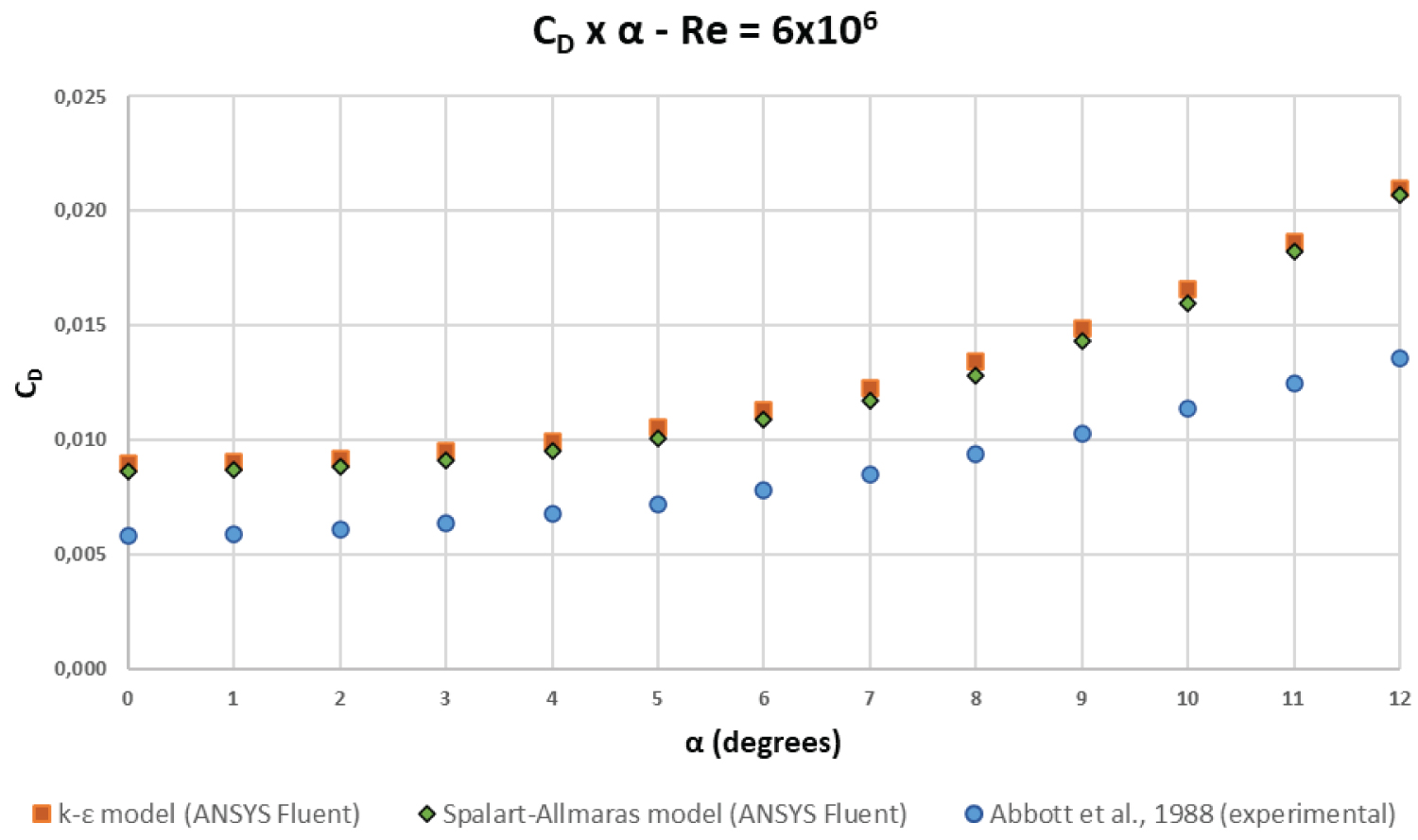
Figure 8: Comparative results for...
Comparative results for - The results for showed physically consistent behavior, despite the imprecision in the results with a margin of error of 50%, probably due to mesh refinement level.
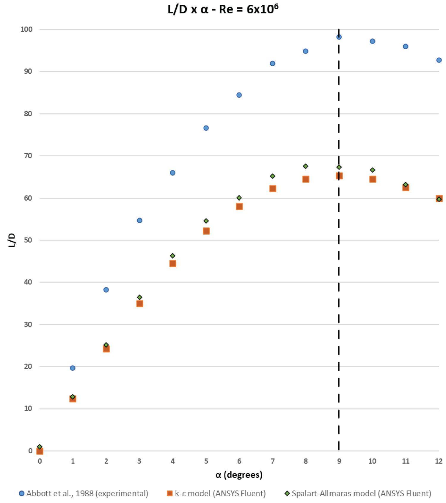
Figure 9: Comparative results for...
Comparative results for L/D - It was observed that at an angle of attack of 9°, the highest lift was achieved with the lowest possible drag penalty.
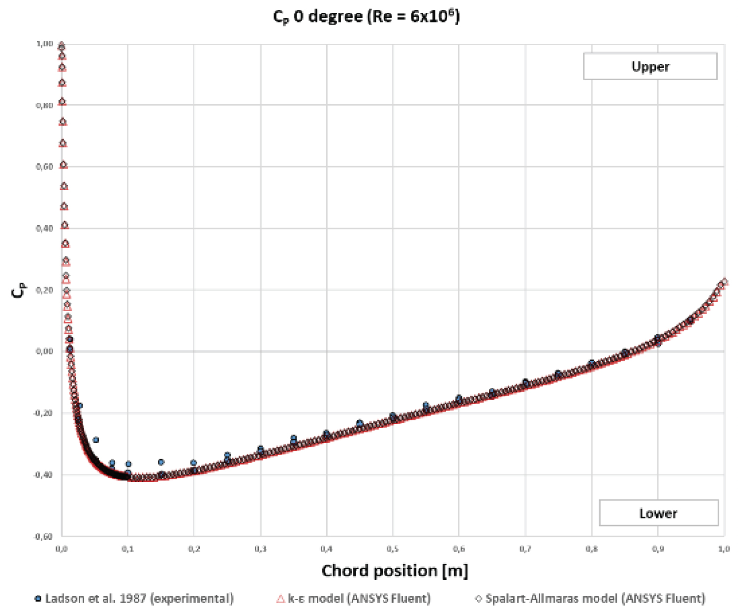
Figure 10: Comparative results for...
Comparative results for (α = 0°) - The symmetric results were due to the geometry of the airfoil.
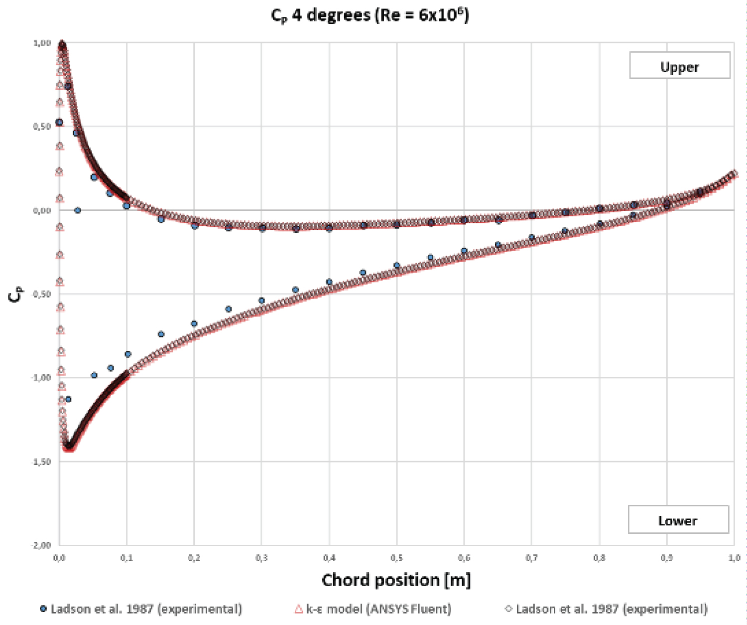
Figure 11: Comparative results for...
Comparative results for (α = 4°) - The area of the graph represents the net lift.
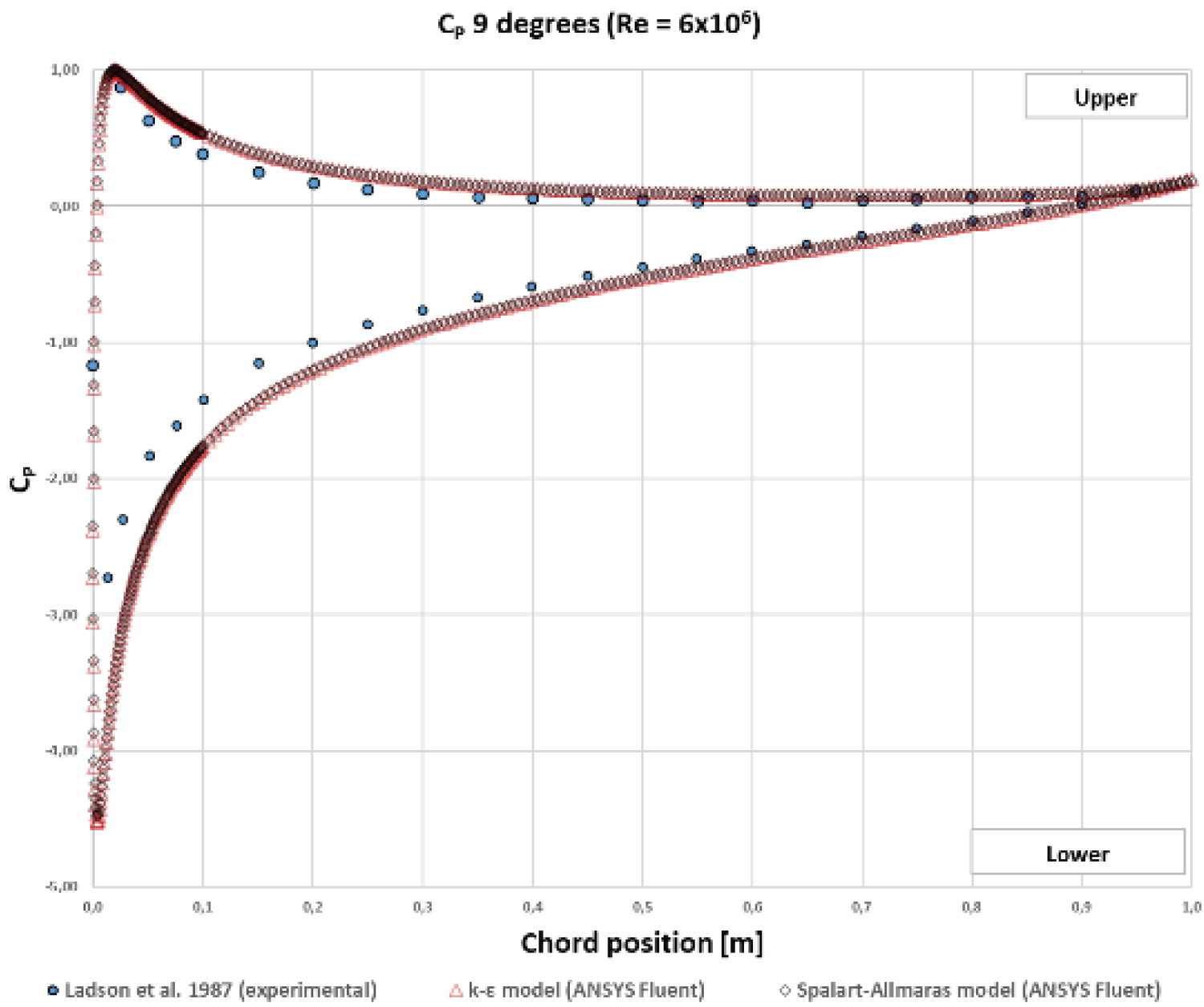
Figure 12: Comparative results for...
Comparative results for (α = 9°) - From this point onwards, the curve tended to shift more towards the upper surface of the airfoil due to the loss of lift.
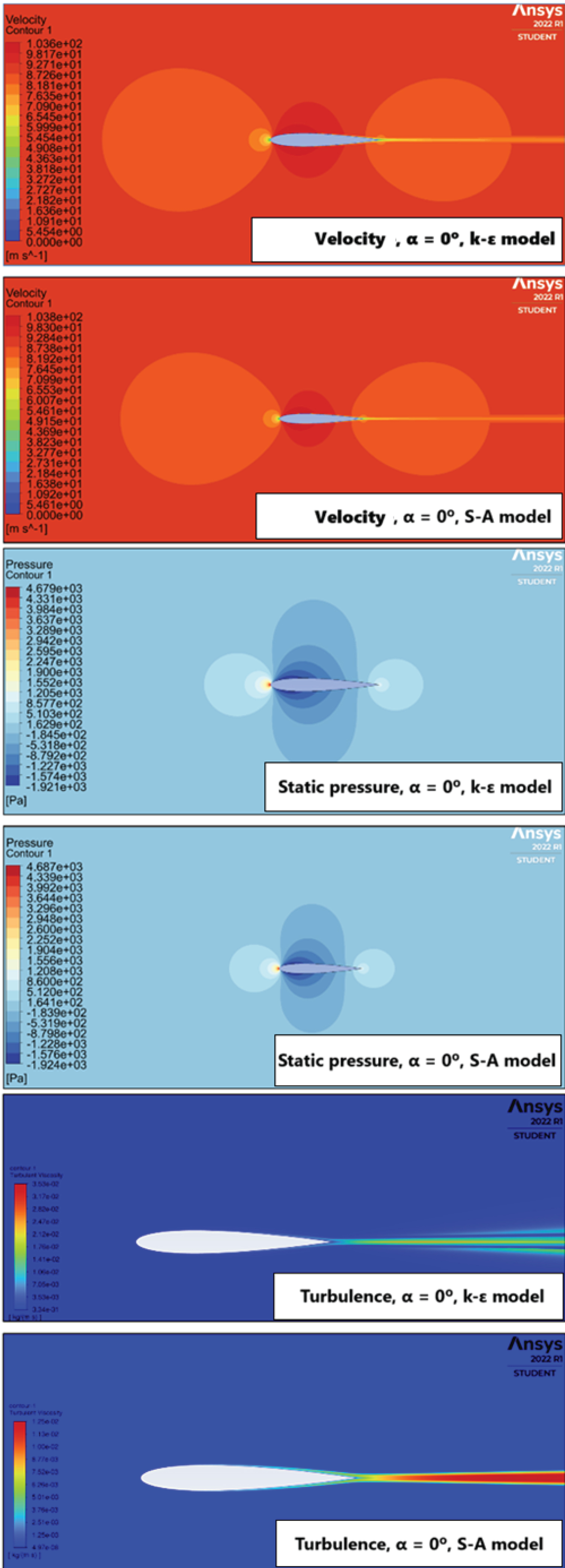
Figure 13: Numerical results for....
Numerical results for α = 0° - The results were symmetric due to the geometry of the airfoil.
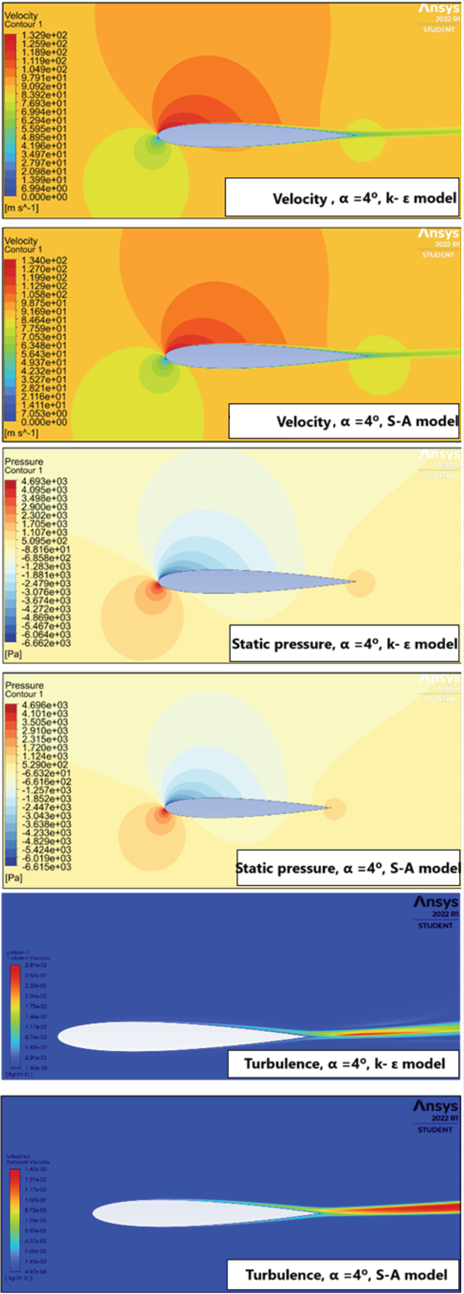
Figure 14: Numerical results for...
Numerical results for α = 4° - Despite the small angle of attack, it was possible to begin observing changes in the behavior of these parameters.
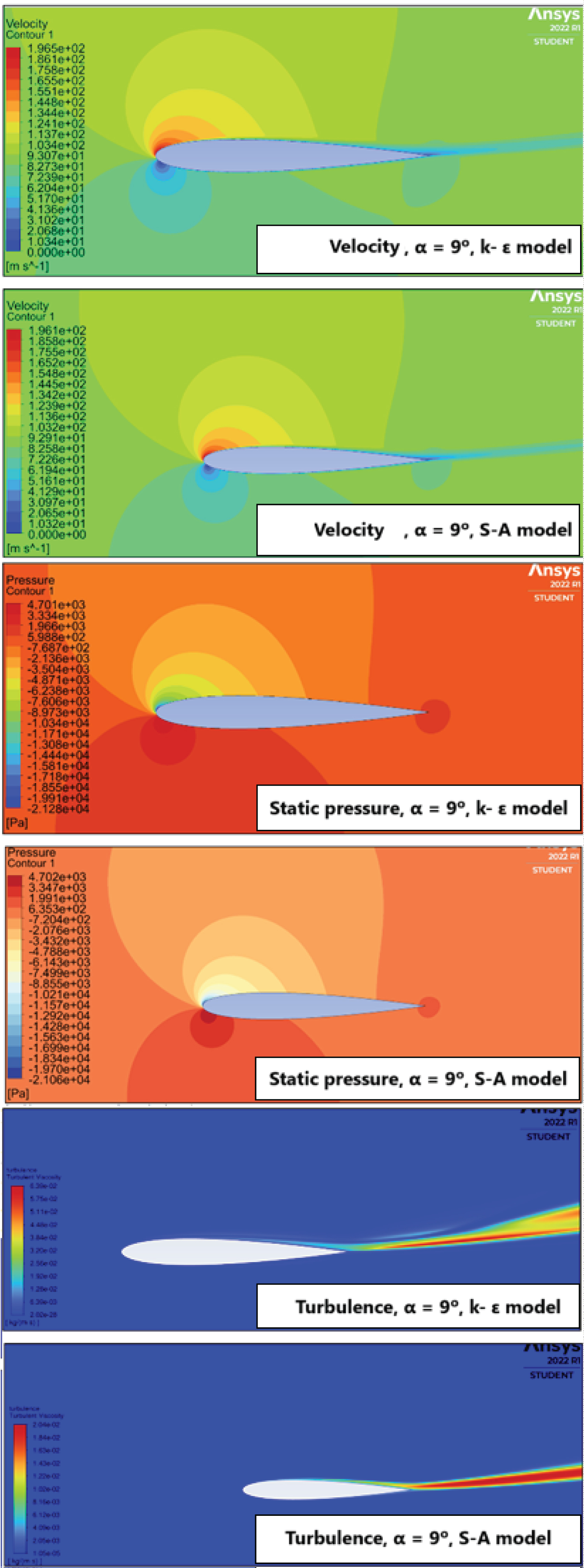
Figure 15: Numerical results for....
Numerical results for α = 9° - At this angle, the profile reaches its maximum efficiency.
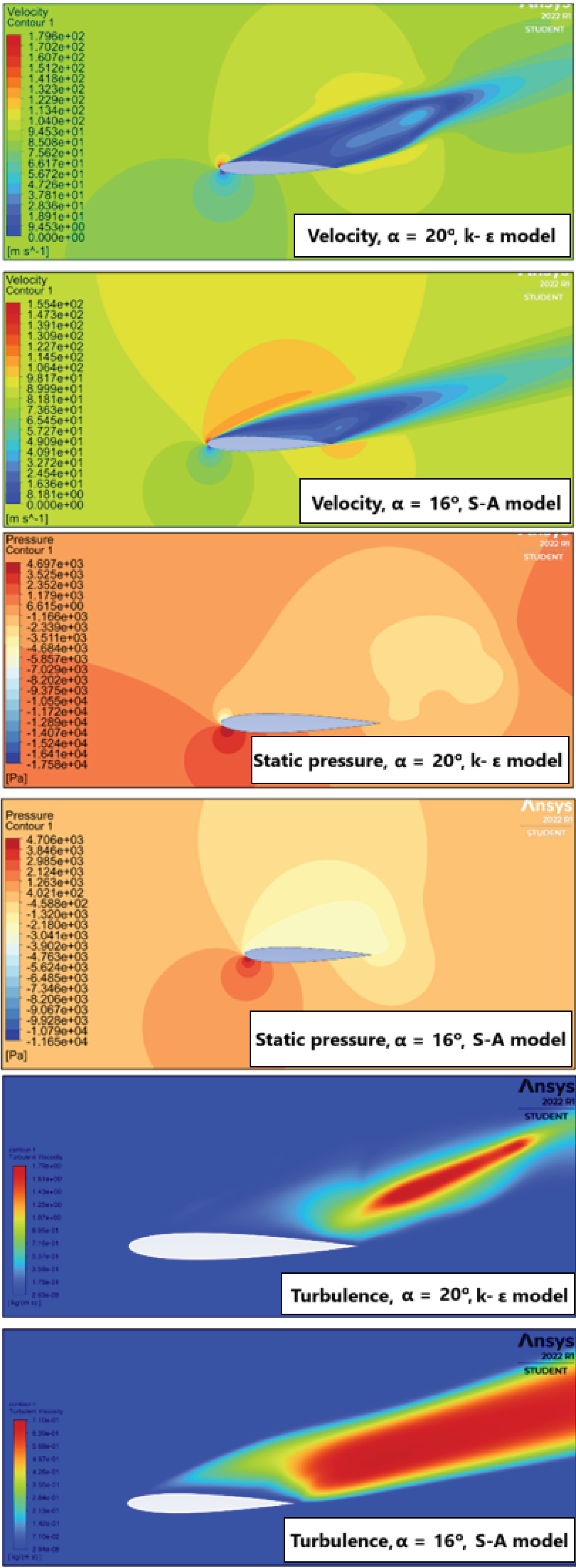
Figure 16: Numerical results for....
Numerical results for α = 16° and 20° - Here, the stall condition is easily identified.
Tables
Table 1: Adopted Boundary Conditions - It was through the boundary conditions that the defined properties of the fluid will be calculated.
References
- Abott IH, Doenhoff AEV (1959) Theory of wing sections: Including a summary of airfoil data. Dover Publications. 462-467.
- Ladson CL, HILL AS, JOHNSON WG Jr (1987) Pressure distributions from high reynolds number transonic tests of an NACA 0012 airfoil in the langley 0.3-meter transonic cryogenic tunnel. NASA Technical Memorandum 100526. 17-22.
- Çengel YA, Cimbala JM (2006) Fluid Mechanics: Fundamentals and applications. Singapore: McGraw-Hill Higher Education.
- Vasconcellos, Guilherme Loyola França (2015) Numerical and experimental study of the flow around a circular cylinder in a wind tunnel at low speeds. Thesis (MSc in Mechanical Engineering) - Pontifical Catholic University of Minas Gerais, Mechanical Engineering Graduate Program, Belo Horizonte: 31-92.
- Patankar SV (1980) Numerical heat transfer and fluid Flow. New York: Hemisphere Publishing Corporation:
- Anderson JD (1998) A history of aerodynamics. Cambridge University Press: Cambridge, 342-345.
- Anderson JD (2011) Fundamentals of aerodynamics. (5 th edn), McGraw-Hill Education:
- Rodrigues LEMJ (2011) Fundamentals of aeronautical engineering. (1 st edn), São Paulo: 23-34.
- Anderson JD (1995) Computational fluid dynamics: The basics with applications. (1 st edn), United States. McGraw Hill: 547.
- Versteeg HK, Malalasekra W (2007) An introduction to computational fluid dynamics: The finite volume method. (2 nd edn), Pearson Education Limited.
- Maliska CR (2004) Heat transfer and computational fluid mechanics. (2 nd edn), Rio de Janeiro. LTC: 399.
- Costa LMF (2018) Numerical investigation of turbulence models in wind flow on suspension bridges. 2018. Dissertation (Master’s in Civil and Urban Construction Engineering) - Polytechnic School of the University of São Paulo. Department of Civil Construction Engineering. São Paulo: 80-87.
- Warsi ZUA (2006) Fluid dynamics: Theoretical and computational approaches. (3 rd edn), Boca Raton. CRC Press.
- Soares CB (2015) Effects of passive attenuators on speed fluctuations in the wind tunnel. Thesis (Doctorate in Mechanical Engineering) - Pontifical Catholic University of Minas Gerais, Postgraduate Program in Mechanical Engineering. Belo Horizonte: 41-44.
- Basha W (2006) Accurate drag prediction for transitional external flow over airfoils. 2006. Thesis (MSc in Mechanical Engineering) – Concordia University. Montreal: 33-53.
Author Details
Augusto Henrique de Miranda Lima* and Luiz Joaquim Cardoso Rocha
PROPEM, Universidade Federal de Ouro Preto, Ouro Preto, Brazil
Corresponding author
Augusto Henrique de Miranda Lima, PROPEM, Universidade Federal de Ouro Preto - UFOP. Rua Nove, 239, Ouro Preto, MG, Brazil.
Accepted: January 27, 2024 | Published Online: January 29, 2024
Citation: Lima AHM, Rocha LJC (2024) Analysis of the Influence of Two Turbulence Models on the Numerical Results of a Computational Fluid Dynamics Simulation for the NACA 0012 Airfoil Profile at Low Speeds. Int J Astronaut Aeronautical Eng 9:066
Copyright: © 2024 Lima AHM, et al. This is an open-access article distributed under the terms of the Creative Commons Attribution License, which permits unrestricted use, distribution, and reproduction in any medium, provided the original author and source are credited.
Abstract
Computational Fluid Dynamics (CFD) techniques are currently an alternative or complementary approach to experimental tests in the field of fluid dynamics. Therefore, this article aims to numerically study the airflow around the NACA 0012 airfoil profile at low speeds using ANSYS ® Fluent and two turbulence models (Spalart-Allmaras and k-ε). The objective is to evaluate the coefficients of lift, drag, and pressure, as well as the lift-to-drag ratio and turbulent wake distribution. The results were considered acceptable through experimental research by Abbott, et al. [1] and Ladson, et al. [2] and showed promising results (C L with an error margin below 5% and maximum aerodynamic efficiency L/D at α = 9°), although they are physically coherent but not as precise (C D demonstrated an error margin of 50%). It was also observed that the Spalart-Allmaras model exhibited better physical coherence in the turbulent wake distribution results compared to the k-ε model, indicating that the latter is not recommended for simulations subjected to adverse pressure gradients.
Keywords
CFD, Lift, Drag, NACA 0012, Spalart-Allmaras, k-ε
Introduction
According to Çengel [3], fluid mechanics is a scientific field dedicated to the study of the behavior of fluids at rest and in motion, as well as the interaction between fluids and solids. The experimental approach involves tests and direct measurements, while the analytical approach seeks to solve differential or integral equations using Computational Fluid Dynamics (CFD). These approaches complement each other and are essential to ensure the accuracy of computational techniques.
Vasconcellos [4] highlights that recent research has focused on studying the flow around different surfaces with relevant applications in the civil, automotive, and aerospace industries. Wind tunnels are often used in the experimental approach to simulate flow conditions, while the analytical approach employs numerical methods with the assistance of CFD. The choice between approaches depends on the problem analysis and their specific advantages, and both are essential for enriching research.
According to Patankar [5], the discussion between experimental and computational approaches does not seek to privilege one over the other but rather acknowledges that both play important roles in fluid mechanics’ research. It is essential to analyze the specific problem at hand and consider the advantages of each approach. The author argues that these methods should be seen as complementary, with experimental data playing a crucial role in verifying the results obtained through the computational approach.
Therefore, in this article, a computational numerical analysis was conducted using ANSYS ® Fluent to investigate the flow around the NACA 0012 airfoil profile (2D) at low speeds using two turbulence models, namely Spalart-Allmaras and k-ε. The profile was chosen because of its symmetrical and uncomplicated geometry, as well as the reasonable amount of research and analysis already carried out and available for consultation.
The aim was to study the drag and lift coefficients (C D and C L ) as a function of the angle of attack (α) and to evaluate the stall behavior of the airfoil as a function of the distribution of turbulence around it using two different turbulence models (Spalart-Allmaras e k-ε realizable). In addition, the pressure coefficient (C P ) as a function of chord length was also evaluated for certain angles (α = 0°, 4° and 9°), as well as the lift-to-drag ratio (L/D) for this airfoil profile. Last but not least, the results were compared through empirical data from Ladson, et al. [2] and Abbott, et al. [1] in order to legitimize these previously mentioned parameters. This reinforces the importance of the complementary nature between the analytical and experimental approaches.
Airfoil profiles
Airfoil profiles significantly influence the performance and stability of aircraft. The geometry of the airfoil, including its shape and thickness, affects the aerodynamic characteristics of the airflow around it, leading to flow separation due to adverse pressure gradient, resulting in a wake of viscous turbulence.
The NACA (National Advisory Committee for Aeronautics) four-digit series profiles were developed based on theoretical and experimental studies, and the nomenclature of these profiles indicates the maximum camber, the position of the maximum camber, and the maximum thickness [6]. The aim of this research was the NACA 0012 airfoil profile (see Figure 1), characterized as a symmetric airfoil with zero camber that follows the centerline, with a thickness of 12% of the chord length.
According to Anderson [7], the drag force F D and lift force F L are expressed through coefficients (C D and C L ) that depend on the fluid density, the chord length of the airfoil (for two-dimensional bodies), the flow velocity, and the airfoil geometry. These relationships can be described by Equations (1.1) and (1.2), which are written in terms of dynamic pressure and reference area.
According to Rodrigues [8], the aerodynamic efficiency of an airfoil can be represented by the lift-to-drag ratio (L/D) as a function of the angle of attack (α). The study of this parameter is of utmost importance for aircraft performance, as it allows identifying the angle at which the airfoil can generate the highest lift with the least possible drag.
Boundary layer
Anderson [7] and Çengel [3] say that the boundary layer is a region adjacent to the surface of an aerodynamic body where viscous effects are present. It exhibits a high velocity gradient, and its development results in friction drag. The difference between laminar and turbulent flow within the boundary layer affects the aerodynamics, with turbulent flow being less prone to separation due to its higher average velocity near the surface, thereby resisting adverse pressure gradients more effectively (see Figure 2).
Mathematical model of the physical problem
In this research, the flow of atmospheric air was considered as a Newtonian fluid, incompressible (with constant density ρ ) and isothermal (with constant viscosity). The flow flows within a fixed arbitrary control volume, bounded by a control surface, and assumes a steady-state hypothesis with a Mach number below to 0.3.
According to Anderson [9], typical aerodynamic flows can be described by the governing equations for fluid dynamics, including the continuity equation and the momentum equation too. Refer to Equations (1.3) to (1.5) below.
Where represents the effective viscosity of the fluid, P is the static pressure and, are the source terms arising from field forces in each direction, in this case, the gravitational force.
Computational fluid dynamics
Computational Fluid Dynamics (CFD) employs numerical methods to solve partial differential equations and study the behavior of fluids. According to Versteeg and Malalasekera [10], all CFD codes have three main phases in their construction, namely, pre-processing, solving, and post-processing, as illustrated by the block diagram in Figure 3.
Finite volume method
The finite volume method is an approach used in the analysis of fluid flow, where the computational domain is divided into finite control volumes. Through a conservation balance of the property in each volume, approximate equations are obtained. Maliska [11] emphasizes the importance of satisfying conservative principles at a discrete level during fluid flow analyses. Patankar [5] mentions that the differential equations governing fluid flow, heat transfer, and mass transfer phenomena can be rewritten in a generalized form known as the General Transport Equation, as shown in Equation (1.6).
Where ϕ is the instantaneous property of the fluid (dependent variable), Γ is the diffusive coefficient, and S is the source term.
Numerical methods discretize the differential equations through a discretization of the domain and the equations. The finite volume method is a numerical method that approximates the transport equations, enabling the computational resolution of the Navier-Stokes equations. By performing the integral over the entire domain, we obtain the discretized General Transport Equation as shown in Equation (1.7) [5].
Where , , and are the coefficients distributed to the neighboring volumes around the control volume P, b is the source term in its linearized form and , , , and are the properties under study for the variables at each nodal point of the control volume mesh.
The solution of this system of algebraic equations must be obtained through an iterative process due to the nonlinearity contained in the equations, not to mention that they are usually coupled with other equations that model, for example, turbulence.
RANS turbulence methodology
The RANS (Reynolds Averaged Navier-Stokes) methodology separates the instantaneous properties of a fluid into a temporal average and a fluctuation. The temporal average of a function is calculated over time, while the fluctuation is the difference between the instantaneous property and its temporal average [3].
According to Costa [12], there are several turbulence models within the RANS methodology, which vary according to the number of additional equations needed to model the phenomenon. In this research, the one-equation Spalart-Allmaras model and the two-equation k-ε model were used to model the turbulence. It is important to mention that most researchers avoid using the k-ε turbulence model in CFD simulations for airfoils because this model does not work well in the presence of an adverse pressure gradient. Therefore, this article proposes using this turbulence model since the NACA 0012 airfoil stall from the trailing edge. In other words, the adverse pressure gradient is not as severe at the leading edge. It was therefore hoped to achieve good results for this turbulence model at low angles of attack - and not at higher angles, close to the stall point.
Spalart-Allmaras model: The Spalart-Allmaras model is widely used in the analysis of aerodynamic flows, especially in aerospace applications with adverse pressure gradients. Although it is effective in these cases, its use in certain situations, such as flows in circular jets, can result in significant errors. This model employs a transport equation to model the turbulent kinematic viscosity, which is a modified form of the actual viscosity, especially in regions near the wall where viscous effects are significant [13].
Basha [14] reports that this model presents a single transport equation to model the turbulent kinematic viscosity . Versteeg and Malalasekera [10] show that the Reynolds stress tensor as well as the transport equation for can be described by Equations (1.8) and (1.9).
Where , , , are constants, is the local mean vorticity, and is a wall-damping factor. This model can be interpreted as follows: The convective transport rate of is equal to the diffusive transport of plus the difference between the generation and dissipation rates of in the control volume.
K- ε model: The two-equation k-ε model is a commonly used approach for turbulence modeling in computational fluid dynamics (CFD) simulations. Its two transport equations describe the turbulent kinetic energy (k) and the rate of turbulent kinetic energy dissipation (ε).
According to Warsi [15], the Reynolds stresses are modeled, and the turbulent viscosity is expressed in terms of turbulent kinetic energy, k, and the rate of turbulent kinetic energy dissipation, ε, as shown in Equation (1.10).
Where is a dimensionless constant. As explained by Vasconcellos [4], when applying this equation to solve a CFD problem, the turbulent viscosity receives two additional variables. In order to solve it, two new equations are incorporated, namely one for k and another for ε, as shown in Equations (1.11) and (1.12).
Where , , , and are constants representing the k-ε model. Versteeg and Malalasekera [10] explain that the first term represents the convection transport of k or ε, the second term is the net rate of diffusive transport of k or ε, and the last two terms represent the production and dissipation rate of k or ε within the control volume.
Materials and Methods
In this study, the fundamental assumptions and the boundary conditions for representing the proposed physical phenomenon were defined according to Table 1.
The assumptions included an isothermal, incompressible, and steady-state flow, with the fluid being considered as a Newtonian fluid (atmospheric air). The adopted definitions for the NACA 0012 airfoil profile included a chord length of 1 m. Finally, the boundary conditions in the fluid dynamics simulations consisted of no-slip at the airfoil surface, an impermeable wall, inviscid and irrotational external flow, and an axisymmetric flow with respect to the z-coordinate.
The procedures followed the block diagram illustrated in Figure 4 and were performed using hardware equipped with the Windows ® 11 Home 64-bit operating system, Intel ® Core ™ i9-12900H CPU @2.50 GHz processor, 32 GB RAM, and NVIDIA ® GeForce ® RTX 3060 dedicated graphics card. Additionally, in this study, the numerical analysis was conducted using the ANSYS ® software, Academic Student version 2022 R1, and its Workbench platform, which offers a variety of applications used for this computational analysis. Although the student license has limitations in mesh generation (512k elements), it provides the same quality as commercial solutions. The Airfoil Tools platform database was used to assist in constructing the NACA 0012 airfoil geometry.
All the execution steps in the software were carried out according to the block diagram presented in Figure 5.
The generated meshes (see Figure 6) had a C-grid format, which allowed for better fitting to the leading and trailing edges of the airfoil. After testing the independence of the meshes, it was observed that mesh 1 was very coarse and that the results of the independence test for mesh 2 and 3 were not that far apart, but the processing time for mesh 3 was much longer as this one was too much fine. Therefore, it was considered for this research the mesh B (medium mesh), which consisted of 304,000 elements and 305,220 nodes.
Results and Discussion
In this chapter, the numerical results obtained using the Spalart-Allmaras and k-ε turbulence models were verified through comparison with Abbott, et al. [1] and Ladson, et al. [2] experiments. The following variables were analyzed for the NACA 0012 airfoil at low speeds:
• Drag coefficients C D as a function of angle of attack (α).
• Lift coefficients C L as a function of angle of attack (α).
• Stall behavior of the airfoil based on the distribution of turbulence around it.
• L/D curve to identify the maximum efficiency of the airfoil.
• Pressure coefficient C P as a function of chord length for α = 0°, 4°, and 9°.
Verification of numerical results
Regarding the coefficient of lift , it was observed that the numerical results obtained were very close to the empirical results for 0° < α < 12° (error margin below 5%). However, for α > 12°, larger differences were observed due to the strong pressure gradient (see Figure 7). was reached for α = 15° and 18° in the Spalart-Allmaras and k-ε realizable models. This is characterized as the profile's stall point.
Similarly, the results obtained for the coefficient of drag C D in ANSYS ® Fluent were compared with the experimental results of Abbott, et al. [1] in a wind tunnel. The error margin was around 50% for 0° < α < 12°, as illustrated in Figure 8.
Regarding lift-to-drag ratio, it was also found that the optimum point on the L/D curve for the NACA 0012 airfoil was reached when α was 8 degrees for the Spalart-Allmaras model and when α was 9 degrees for the k-ε model, as shown in Figure 9. Despite the small difference, the L/D curve indicates that, in this condition, the numerical models used were qualitatively consistent with the experimental results of Abbott, et al. [1], with a slight quantitative deviation from their results since the 9 degrees provides the highest lift with the least drag penalty, i.e. the maximum aerodynamic efficiency of the airfoil. However, beyond this angle, the pressure gradient increases rapidly and, if not controlled, can lead to boundary layer separation and stall of the airfoil.
Finally, the analysis of the distribution of the pressure coefficient C P along the NACA 0012 airfoil for different angles of attack showed that the numerical results were close to the experimental data, which made the numerical model acceptable for this research. For an angle of attack of 0 degrees, the pressure was nearly the same on the upper and lower surfaces of the airfoil due to symmetry.
On the other hand, for α = 4° and α = 9°, there is a slight fluctuation between the numerical results and the experimental data on the lower surface of the profile. However, it is precisely because of this difference of pressure that the profile produces the net lift force. Lastly, as the angle of attack increased, there was an even greater pressure difference between the upper and lower surfaces, resulting in the lift force (see Figure 10, Figure 11 and Figure 12).
Distribution of velocity, static pressure, and turbulent wake on the airfoil
Once the numerical model has been considered accepted, the distribution of velocity, static pressure, and turbulent wake around the NACA 0012 airfoil was evaluated under the conditions of the k-ε and Spalart-Allmaras turbulence models, as shown in Figure 13, Figure 14, Figure 15 and Figure 16.
When analyzing the results for different angles of attack, a symmetric pattern was observed in the graphs for α = 0°, with a laminar boundary layer transitioning to a turbulent regime beyond half of the chord length (see Figure 13).
From 4 degrees, as shown in Figure 14, it was possible to observe an increase in lift production and a displacement of the stagnation point towards the lower surface of the airfoil, as well as an increase in velocity and thickness of the boundary layer on the upper surface.
For α = 9 degrees, Figure 15 shows that the velocity reached its maximum value at the leading edge, the static pressure increased, the turbulent wake was more intense at the trailing edge, the transition of the boundary layer occurred earlier, and a greater thickness of the boundary layer on the upper surface was observed.
Finally, Figure 16 shows the parameters for angles of attack α equal to 16 degrees (Spalart-Allmaras model) and 20 degrees (k-ε model). These were the exact moments that followed the stall of the airfoil (notice the significant increase in turbulent wake and the complete disorder downstream of the airfoil's upper surface).
Conclusions
In this paper, numerical simulations of airflow over the NACA 0012 airfoil were conducted. The results indicated that increasing the angle of attack leads to higher drag, with the maximum aerodynamic efficiency obtained at α = 8 degrees (Spalart-Allmaras model) and α = 9 degrees (k-ε model). The comparison of the results for the pressure coefficient showed agreement with experimental studies, highlighting that the airfoil's upper surface exhibits significantly higher static pressure distribution compared to the lower surface. The need to refine the chosen mesh (medium mesh) in order to predict the drag coefficients can certainly be inferred from the mesh sensitivity results. This is due to the fact that these coefficients exhibited a margin of error of 50% for α from 0 to 12 degrees, contrasting with a margin of error below 5% for the lift coefficients in the angle of attack range of 0 < α < 9 degrees.
From the simulation of the NACA 0012 airfoil, it was observed that when the angle of attack was 0 degrees, the turbulence wake distribution was very accurate and reliable for both turbulence models. However, as the value of α increased, it was noted that the turbulence for the k-ε model always showed greater oscillations compared to Spalart-Allmaras model, even for low values of α (adverse gradient not severe). Furthermore, after the airfoil stall, the boundary layer separation was not as evident for the realizable k-ε model, even considering that it still had a stall angle that was 2 degrees greater than Abbott's [1] experimental data.
As a suggestion for continuing and complementing this research, it would be interesting to redo the same CFD analyses considering the flow as compressible. In this way, the effects of compressibility and the formation of the shock wave and its expansion would be considered in the research. It is also suggested that more precise techniques be used, such as LES and DNS, combined with a finer mesh.

