
International Journal of Earth Science and Geophysics
(ISSN: 2631-5033)
Volume 4, Issue 1
Review Article
DOI: 10.35840/2631-5033/1818

Article Formats
A Review of the Current Understanding in the Study of Geomagnetic Storms
Table of Content
Figures
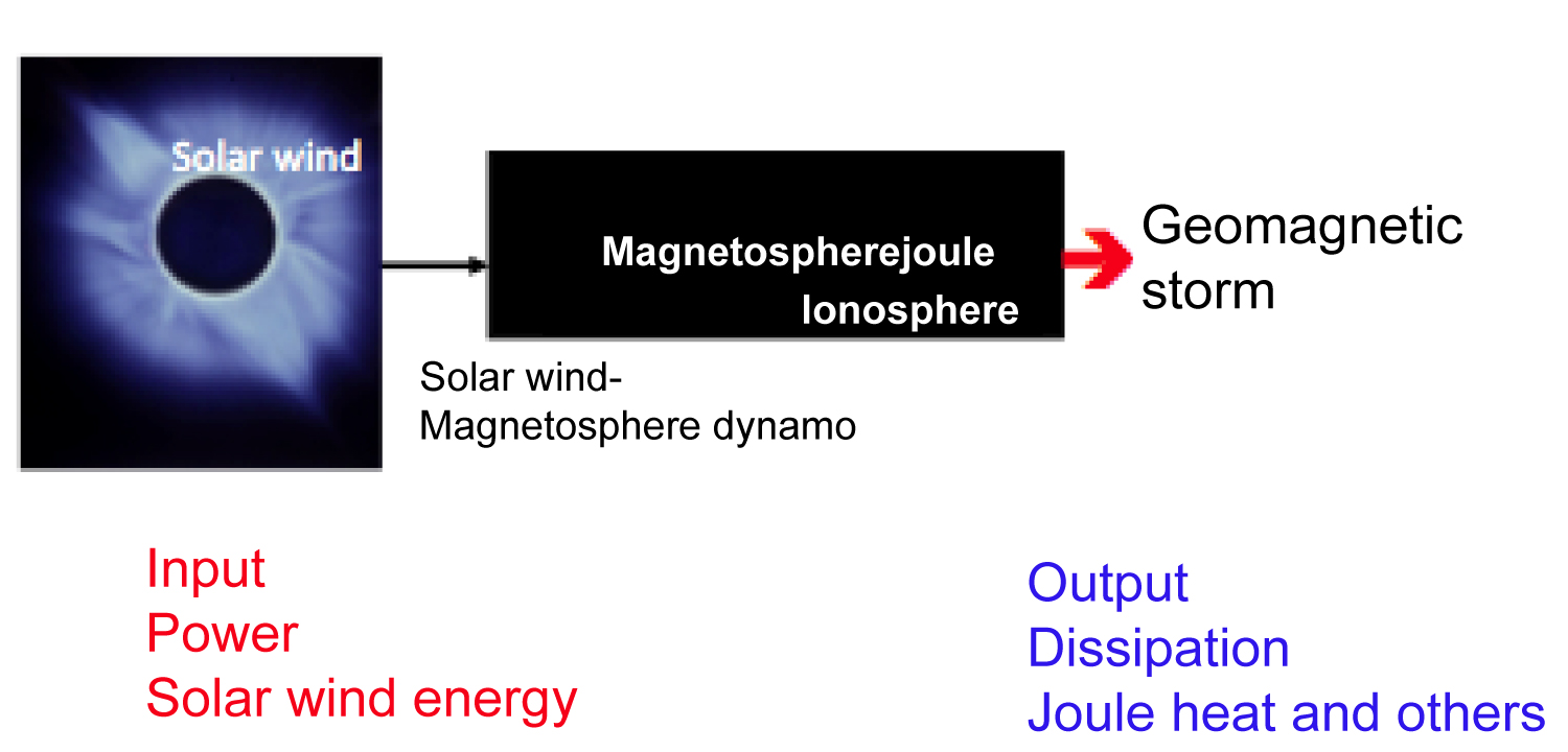
Figure 1: The relationship among the sun (corona)...
The relationship among the sun (corona), the solar (plasma) wind, the magnetosphere/ionosphere and geomagnetic storms. This chain of processes can be considered as an input-output problem, in which the solar wind energy is converted into electric power by the solar wind-magnetosphere dynamo which generates the three storm current systems [29].

Figure 2: Low and middle latitude magnetic records...
Low and middle latitude magnetic records from the African, Middle East, Asian and American sectors during the geomagnetic storm of April 17-18, 1965 [39]. The common features in the records are the storm sudden commencement, ssc (a sudden stepwise increase), the initial phase and the main phase decrease and the recovery phase. Note that main phase decrease was larger in the Middle East and Asian sectors (the evening sector) in this storm; see Section 4.
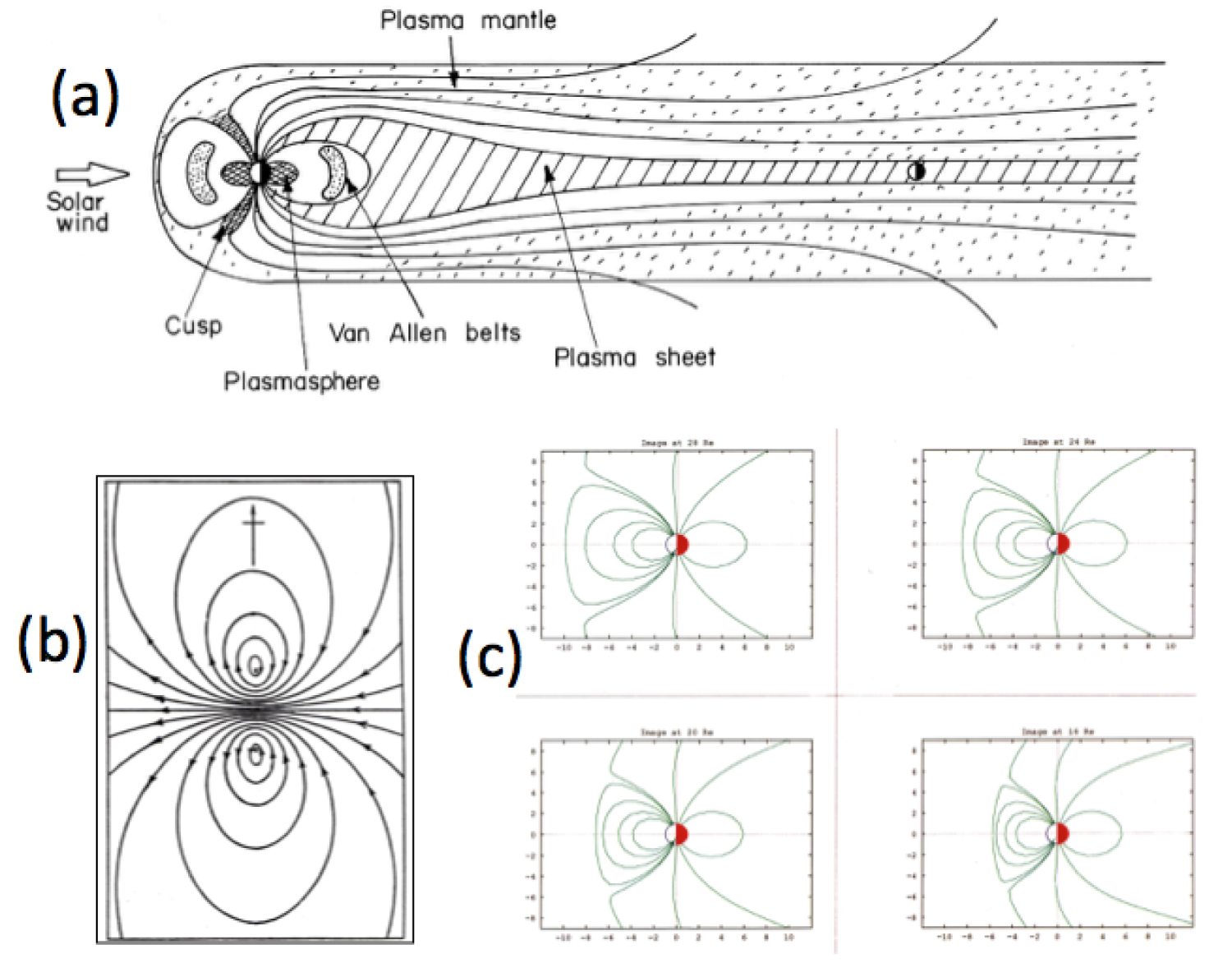
Figure 3: a) The permanent structure of a comet-shaped...
a) The permanent structure of a comet-shaped magnetosphere, including several major internal structures, the plasma mantle, cusp, plasmasphere, Van Allen belt and plasma sheet; b) The Chapman-Ferraro current (the C-F current) induced on the front of the advancing solar plasma flow [two-dimensional] [1]; c) The current at the front of the plasma advancing toward the earth compresses the magnetosphere.
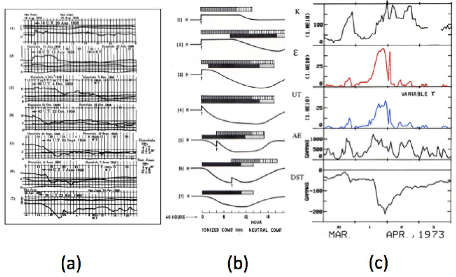
Figure 4: a) A great variety of the development of...
a) A great variety of the development of geomagnetic storms; actually the top one was once called 'si, sudden impulse' and last one was called 'Sg (gradually commencing) storm', and both had been removed from the list of storms; b) An effort to explain the variety of development in terms of neutral hydrogen atoms; c) From the top, the kinetic energy flux (K), the power generated by the solar wind-magnetosphere dynamo (ε), the total energy dissipated in the magnetosphere and the ionosphere (UT) during the geomagnetic storm of March 31 - April 3, 1973. The intensity of geomagnetic storms is represented by two indices; the Dst index is the average main phase decrease and the AE index represents the intensity of the auroral electrojet; both geomagnetic indices AE and Dst are used to compute the dissipation rate during the storm.
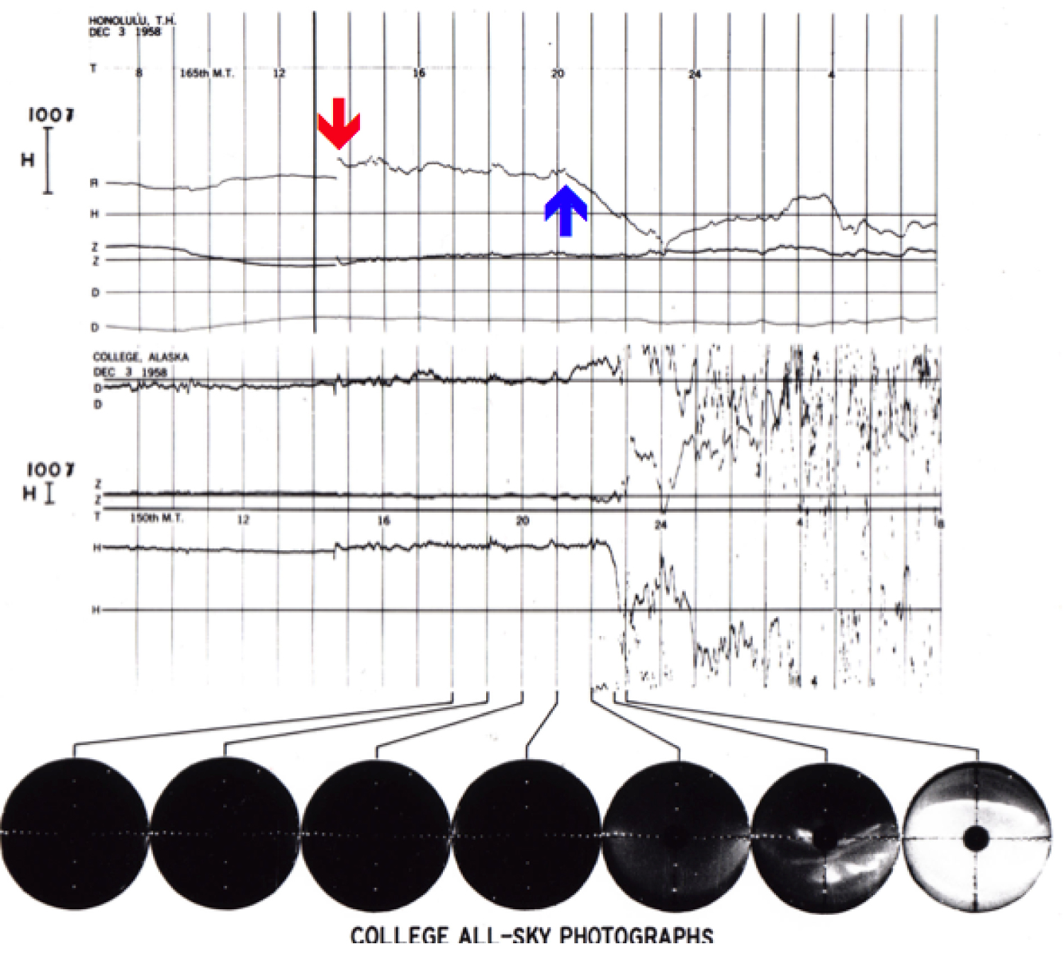
Figure 5: An example of the simultaneous onset of...
An example of the simultaneous onset of both the main phase of the December 3, 1958 storm (recorded in Hawaii) and auroral activities (all-sky camera photographs and polar magnetic disturbance recorded in Fairbanks). The ssc (red arrow) and the onset of the main phase onset (blue arrow) are marked.
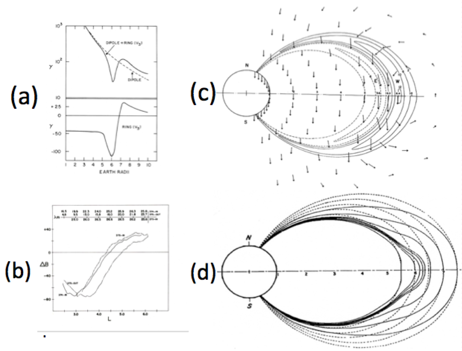
Figure 6: a) The distorted earth magnetic field and...
a) The distorted earth magnetic field and the ring current field as a function of the distance from the earth; b) The first observation of the ring current field [17]; c) The distribution of electric current produced by the trapped positive particles [centered around 6 Re] and the magnetic field [15]. The ring current field near the earth is directed southward, and thus can explain the main phase decrease; d) The distorted magnetic field lines. The figure shows the distribution of the ring current; a weaker current flows eastward in its inner side (E) and stronger current (W) westward in the outer side. The current is mostly the diamagnetic current [40].
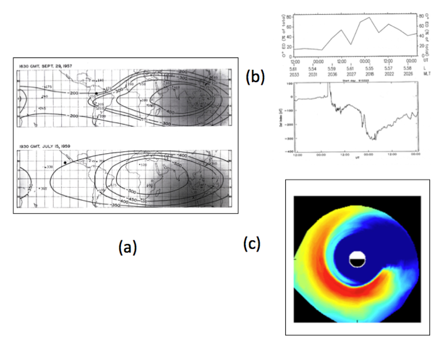
Figure 7: a) Large development of the asymmetry of...
a) Large development of the asymmetry of the main phase during an early epoch of the main phase of the September 20, 1957 and July 15, 1959 storms; the figures show iso-intensity contours of the main phase intensity of the main phase; b) The population of O+ ions and the main phase index Dst; as O+ ions increases, the Dst index responds [21]; c) A simulation study of the formation of the ring current [22]; after being ejected in the midnight sector, O+ ions start to drift westward.
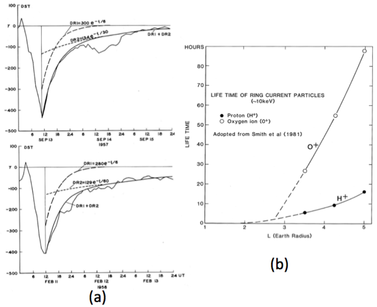
Figure 8: a) Two storms are shown, indicating that...
a) Two storms are shown, indicating that the recovery phase needs two exponential functions to fit the rate of the recovery [24]; b) A very tentative life-time of O+ ions and protons.
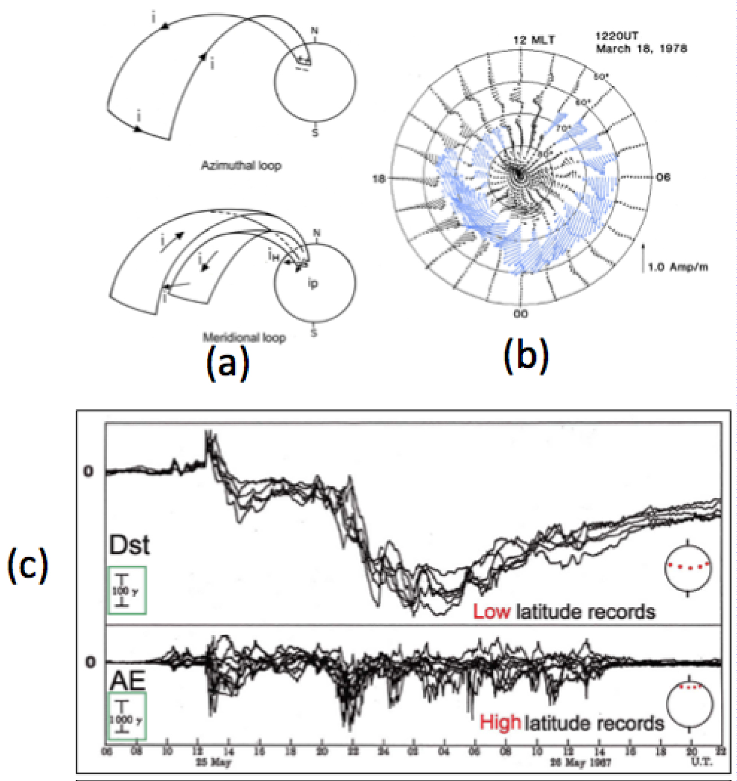
Figure 9: a) The 3-D electric current system...
a) The 3-D electric current system which consists of the azimuthal and meridional components [32]. This current system develops during the expansion phase of auroral substorms; b) The distribution of the ionospheric current during the expansion phase during the maximum epoch, which is caused by the current system in [41]; c) Both low latitude and high latitude magnetic records during the geomagnetic storm of May 25-26, 1967. Note the difference of the scale.

Figure 10: a) Simple two co-rotating structures from...
a) Simple two co-rotating structures from two coronal holes. It is assumed that the velocity of the solar wind has a sinusoidal structure in a longitude-latitude map; b) It shows schematic all the extent of the flows from the coronal holes.
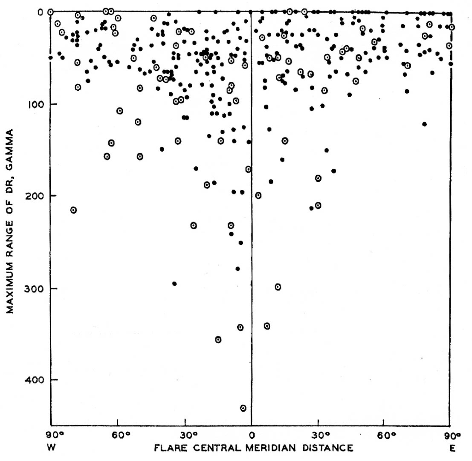
Figure 11: The relationship between the central...
The relationship between the central meridian distance of flare locations and the intensity of the main phase, the Dst (denoted as DR, Gamma = nT) [42].
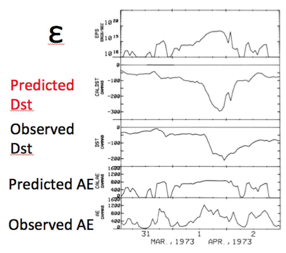
Figure 12: An example to show that once the power...
An example to show that once the power P(= ε) is known, it is possible to predict the geomagnetic storm index Dst and the substorm index AE [43]; in this case, the AE index is saturated. The predicted AE and Dst indices are determined empirically by examining their relationship with ε.
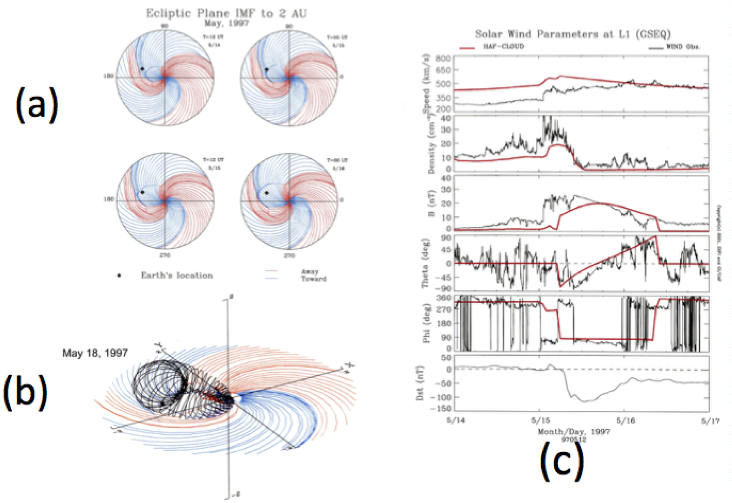
Figure 13: a) The propagation of the shock wave in...
a) The propagation of the shock wave in interplanetary space (sun at the center, the earth is indicated as a dot) associated with the May, 1997 solar flare; [37]; b) Reconstruction of the helical magnetic structure associated with the same flare event [38]; the earth is indicated by a dot; c) Comparison of the results between the observation and the reconstructed helical structure, together with the standard solar wind quantities [38]; θ = -(theta-90°).
References
- Chapman S, VCA Ferraro (1931) A new theory of magnetic storms. I Initial Phase Terr Mag 36: 77-97.
- Cahill LJ, PG Amazeen (1963) The boundary of the magnetospheric field. J Geophys Res 68: 1835-1843.
- Ness NF, CS Sceace, JB Seek (1964) Initial results of the Imp 1 magnetic field expiment. J Geophys Res 69: 3531-3569.
- Chapman S, VCA Ferraro (1933) A new theory of magnetic storms. II Main Phase Terr Mag 38: 79-96.
- Axford, WI, CO Hines (1961) A unifying theory of high latitude geophysical phenomena and geomagnetic storms. Canadian J Phys 39: 1433-1464.
- Dungey JW (1961) Interplanetary magnetic field and the auroral zone. Phys Rev Lett 6: 47-48.
- McIlwain CE (1974) Substorm injection boundaries. Magnetospheric Physics. BM MCormac, D Reidel Pub. Co., Dordrecht-Holland, 143.
- Akasofu SI, S Chapman (1963) The development of the main phase of magnetic storms. J Geophys Res 68: 125-129.
- Akasofu, SI (1964) The neutral hydrogen flux in the solar plasma flow-I. Planet Space Sci 12: 905-913.
- Fairfield DH, LJ Cahill Jr (1966) Transition region magnetic field and polar magnetic disturbances. J Geophys Res 71: 155-169.
- Akasofu SI (1978) The interaction between a magnetized plasma flow and a magnetized celestial body: A review of magnetospheric studies. Space Sci Rev 21: 489-526.
- Akasofu S (1977) Physics of Magnetospheric Substorms.D. Reidel Pub. Cp., Dordrecht-Hollamd, 599.
- Alfven H (1950) Cosmical Electrodynamics, Oxford Univ.
- Akasofu SI, S Chapman (1961) The ring current, Geomagnetic disturbances and the Van Allen radiation belts. J Geophys Res 66: 1321-1350.
- Akasofu SI, JC Cain, S Chapman (1961) The magnetic field of a model radiation belt, numerically computed. J Geophys Res 66: 4013-4026.
- Frank LA (1967) On the extraterrestrial ring current during geomagnetic storm. J Geophys Res 75: 3753-3767.
- Cahill LJ (1966) Inflation of the inner magnetosphere during a magnetic storm. J Geophys Res 71: 4505-4519.
- Akasofu SI, S Chapman (1964) On the asymmetric development of the magnetic fields in low and middle latitudes. Planet and Space Sci 12: 607-626.
- Shelley EG, Johnson RG, Sharp RD (1972) Satellite observations of energetic heavy ions during geomagnetic storm. J Geophys Res 77: 6104-6110.
- DG Mitchell, SE Jaskulek, CE Schlemm, EP Keath, RE Thompson, et al. (2000) High energy neutral atom (HENA) imager for the IMAGER mission. Space Sci Rev 91: 67-112.
- Daglis IA (1997) Mission study oxygen issue. EOS 78: 245-251.
- Mei-Ching Fok, Thomas E Moore, Pontus C Brandt, Dominique C Delcourt, Steven P Slinker, et al. (2006) Impulsive enhancement of oxygen ions during substorms. J Geophys Res 111: 10222.
- Fok MC (2003) Global ENA simulations. In: JL Burch, Magnetospheric Imaging: The IMAGE Prime Mission. Kluwer Academic Pub, 77-103.
- Akasofu SI, S Chapman, D Venkatesan (1963) The main phase of great magnetic storms. J Geophys Res 68: 3345-3350.
- Kozyra JU, MW Liemohn (2003) Ring current energy input and decay. In: JL Burch, Magneospheric Imaging: The IMAGE Mission. Kluwer Academic Pub, 105-131.
- Birkeland KR (1918) The Norwegian Auroral Polaris Expedition, 1902-1903. 801.
- Stormer C The polar Aurora. Oxford University Press, 403.
- Chapman S (1935) The electric current systems of magnetic storm. Terr Mag 40: 349-370.
- Akasofu SI (2017) Auroral substorms: Search for processes causing the expansion phase in terms of the electric current approach. Space Sci Review 212: 341-381.
- Chapman S, J Bartels (1940) Geomagnetism. Oxford University Press.
- Akasofu SI, S Chapman (1963) Magnetic storms: The simultaneous development of the main phase (DR) and of polar magnetic substorms (DP). J Geophys Res 68: 3155-3158.
- Bostrom RA (1964) A model of the auroral electrojets. J Gophys Res 69: 4983-4999.
- Canfield RC, HS Hudson, DE McKenzie (1999) Sigmoidal morphology and eruptive solar activity. Geophys Res Lett 26: 627-630.
- Akasofu SI (2017) The electric current approach in the solar-terrestrial relationship. Ann Geophys 35: 1-14.
- Burlaga L, E Sitter, F Marini, R Schwenn (1981) Magnetic loop behind an interplanetary shock: Voyager, Helios and IMP 8 observations. J Geophys Res 86: 6673-6684.
- Gosling JT, DN Baker, SJ Bame, RD Zwickl (1986) Bidirectional solar wind electron heat flux and hemispherically symmetric polar rain. J Geophys Res 91: 11352-11358.
- Fry CD, W Sun, CS Deehr, M Dryer, Z Smith, et al. (2001) Improvement to the HAF solar wind model for space weather predictions. J Geophys Res 106: 20985-21001.
- Saito T, W Sun, CS Deehr, SI Akasofu (2007) Transequatorial magnetic flux loops on the sun as a possible new source of geomagnetic storms. J Geophys Res 112: 05102.
- Meng CI, Akasofu (1967) The geomagnetic storm of April 17-18, 1965. J Geophys Res 72: 4905-4916.
- Dessler AJ, EN Parker (1959) Hydromagnetic theory of geomagnetic storms. J Geophys Res 64: 2239-2252.
- Kamide Y (1982) Global distribution of ionospheric and field-aligned currents during substorms as determined from six meridian chains of magnetometers: Initial results. J Geophys Res 87: 8228-8240.
- Yoshida S, SI Akasofu (1965) A study of the propagation of solar particles in interplanetary space: The center-limb effect of the magnitude of cosmic-ray storms and of geomagnetic storms. Plant Spce Sci 13: 435-448.
- Akasofu SI (1981) Energy coupling between the solar wind and the magnetosphere. Space Sci Rev 28: 121-190.
Author Details
Syun-Ichi Akasofu*
International Arctic Research Center, University of Alaska Fairbanks, Fairbanks, USA
Corresponding author
Syun-Ichi Akasofu, International Arctic Research Center, University of Alaska Fiarbanks, Fairbanks, Alaska, USA, Tel: 99775-7340.
Accepted: June 12, 2018 | Published Online: June 14, 2018
Citation: Syun-Ichi A (2018) A Review of the Current Understanding in the Study of Geomagnetic Storms. Int J Earth Sci Geophys 4:018.
Copyright: © 2018 Syun-Ichi A. This is an open-access article distributed under the terms of the Creative Commons Attribution License, which permits unrestricted use, distribution, and reproduction in any medium, provided the original author and source are credited.
Abstract
Geomagnetic storms are the magnetic manifestation of disturbances caused by the impact of solar plasma flows generated by various solar activities. They consist of its onset (called the storm sudden commencement, ssc), the initial, main and recovery phases. Three distinct current systems (the Chapman-Ferraro current, ring current, and auroral electrojet) are generated by the solar wind-magnetosphere dynamo, and their magnetic fields are observed as magnetic disturbances-most intense ones, geomagnetic storms. Research on the processes generating these three current systems has encountered many serious theoretical difficulties, but continuous efforts (both observational and theoretical), unexpected solutions and discoveries, as well as a number of controversies, have led us to the present understanding of geomagnetic storms. However, there are still a number of problems to be solved for a better understanding of geomagnetic storms and the prediction of their occurrence in terms of "space weather prediction", in particular the prediction of the polar angle θ (or IMF Bz) of the magnetic field in coronal mass ejections (CMEs) and co-rotating regions (CIR).
Keywords
Geomagnetic storms, Ring current, Space wheather
Introduction
Solar activities, such as solar flares and coronal holes, produce various effects on the earth. One of them is plasma flows which cause three major current systems in the magnetosphere/ionosphere system, generating three different kinds of magnetic changes (the chapman-Ferraro current, ring current, auroral electrojet), which are observed all together as geomagnetic disturbances, most intense ones-geomagnetic storms.
The energy produced by solar activities is carried by plasma flows and is eventually dissipated as the Joule heat in the ionosphere and by other processes (Figure 1). Thus, in terms of energy flow, this series of processes can be considered as an input-output relationship (problem).
Geomagnetic storms are a worldwide phenomenon. Figure 2 shows a number of magnetic records (the horizontal [north-south] component) from midlatitude and low latitude stations during the April 17-18, 1965 storm. In general, geomagnetic storms consist of the storm sudden commencement (ssc), the initial, main and recovery phases. The ssc is a step-function-like increase (the horizontal or NS component) of the earth's magnetic field (~25 nT), which is followed by the initial phase, which is relatively quiet period for a few hours. After the initial phase, the main phase begins, during which a large southward (reckoned negative) field develops for about 6-10 hours (50-500 nT). During the same period, intense polar magnetic disturbances occur intermittently (often more than 1000 nT), together with a specific auroral activity, called auroral substorms (described in Section 5). The last phase is the recover phase.
Geomagnetic storms, including the accompanying polar magnetic disturbances, are caused by three distinct current systems (except the recovery phase when the current systems subside): (1) The storm sudden commencement (ssc) and the initial phase are caused an enhancement of the Chapman-Ferraro current on the boundary surface of the magnetosphere. (2) The main phase is caused by the ring current around the earth (within the magnetosphere). (3) Polar magnetic disturbances are caused by intense ionospheric currents, called the auroral electrojet. In the following, the present understanding of each current system and its causes are described and discussed.
Storm Sudden Commencement, Ssc: Chapman-Ferraro Current
Chapman and Ferraro [1] was the first to consider the impact of solar plasma flows on the earth's dipole field, and their theory became the first theory of the formation of the magnetosphere and of the storm sudden commencement (ssc). When disturbed solar plasma flows approach toward the earth's dipole, the Chapman-Ferraro (C-F) current is induced on its front surface, and the associated Lorentz force stops its advance. When the advancing front of the plasma stops, the C-F current flows on the boundary of the magnetosphere (a comet-like structure around the earth) and has an effect of "compressing" earth's dipole field; its effect is recorded as a step-function like variation, ssc (Figure 3).
Since we know now that the solar wind is a permanent feature, the magnetosphere and the C-F current are also a permanent feature. The present understanding of ssc is that when disturbed plasma flows arrive, the C-F current is enhanced, and its magnetic field is recorded as ssc; just inside the front boundary, the dipole field is doubled. The magnitude of ssc is proportional to the increased pressure. Chapman-Ferraro's theory had not necessarily been widely accepted until a satellite observation confirmed it 32 years later [2].
Initial Phase: Chapman-Ferraro Current
It is a relatively quiet period of a few hours (on the average) before the main phase onset. This was a great puzzle for many years, because the main phase does not often develop immediately after ssc (signaling the arrival of disturbed solar wind). This puzzle was solved partly by the discovery of the interplanetary shock wave which advances ahead of an intense plasma flow (causing the compression and ssc) before the arrival plasma clouds [coronal mass ejections, CMEs] [3]. The initial phase lasting for a few hours is considered to be the period of the passage of the region between the shock wave and, such as CMEs and co-rotating structure (CIR) (see also Section 6).
Main Phase
The main phase is caused by the ring current around the earth, and its horizontal field intensity (measured by the index called Dst) ranges from 50 nT (weakest storms) to about 500 nT (most intense storms). This field is southward-directed, and because northward-oriented fields are reckoned as positive, the main phase is characterized by a decrease of the earth's magnetic field (Figure 2); note that the observed field is 20% larger than that of the ring current field, because the earth's induction effect is added.
Formation of the ring current belt
Early history
After formulating their theory of ssc, Chapman and Ferraro [4] tried to find the cause of the main phase by considering a ring of current flowing westward within the magnetosphere, specifically a circular motion of charged particles. The immediate problems they faced were: (i) How solar wind plasma particles can enter into the magnetosphere to form the ring current belt (because their theory tells that the plasma simply flows around the magnetosphere) and (ii) How the entered plasma particles can form a ring of electric current.
Entry of solar wind plasma?
Many researchers, including Chapman, had tried to find ways for the solar plasma to enter across the dayside boundary of the magnetosphere, but it was eventually found that the entry of solar wind protons from the front side of the magnetosphere was not possible. Axford and Hines [5] and Dungey [6] proposed that the solar plasma particles get into the magnetosphere from backside and are subsequently convected and injected into the ring current belt. This injection process was observed and confirmed at the geosynchronous location by McIlwain [7]. It was later found that O+ ions are injected into the magnetosphere and then convected back to the ring current (see Section 4.3).
Importance of the interplanetary magnetic field (IMF)
In examining the relationship among the storm sudden commencement (ssc), initial and main phases, it was found that geomagnetic storms develop in a great variety of ways. In some cases, a large ssc and long-lasting initial phase do not produce the main phase [called 'si']. In some other cases, storms develop even without ssc (such storms are called Sg [gradually commencing] storms). Figure 4a shows this great variety. In an effort to try to understand the variety, Akasofu and Chapman [8] concluded that the solar wind must contain something "unknown", other than protons and electrons in the solar wind; Akasofu [9] considered once that as the "unknown", the solar wind contains neutral hydrogen atoms which can penetrate through the magnetospheric boundary (without causing ssc) and become ring current protons by the charge exchange process; Figure 4b shows an effort to explain the variety in terms of the hypothetical distribution of hydrogen atoms in the plasma flows. However, it was considered that the solar wind would not contain enough neutral hydrogen atoms.
The author found examples of storms during which the main phase and the intense auroral activities develop simultaneously well after the ssc. Figure 5 shows such an example. This delay of the onset 6 hours after the ssc is not easy to explain.
Chapman presented this example during the first solar wind conference in 1964. There was a discussion session after his presentation: (1) W. I. Axford stated in part: "This particular storms to support very well the suggestion that interchange motions play dominant role in magnetic storms". (2) J. W. Dungey stated in part: "I think main phase of the storm is caused by something in the high-pressure gas, and the best guess is a strong southward interplanetary field. However, this is a question still to be answered".
Dungey's suggestion was then confirmed by Fairfield and Cahill [10] who stated that the "unknown" factor inferred by [8] is the southward component of the interplanetary magnetic field (IMF), which is denoted now as -Bz; In Figure 4b, we can replace the neutral hydrogen by IMF -Bz. The onset of the main phase is determined by the arrival of -Bz, not the arrival of the plasma flow (signaled by ssc).
This discovery of the IMF -Bz has led eventually to our understanding that the solar wind-magnetosphere interaction constitutes a dynamo which generates the power needed for producing the ring current and auroral electrojet. Figure 4c shows that the kinetic energy (K) carried by the solar wind alone cannot cause geomagnetic storms. On the other hand, the output as the total dissipation (UT) varies in a way similar to the power (ε) of the solar wind-magnetosphere dynamo [11].
The power P (ε = P/8π) in Figure 4c of the solar wind-magnetosphere dynamo is defined by the Poynting flux P (erg/s) in terms of observable quantities ([12] Section 1.4) and is given by:
Where V and B are the solar wind speed and the intensity of the IMF, respectively, and S = sin4(θ/2)l2 where θ is the polar angle of the IMF and l is 5 Re (Re = The earth's radius).
Nature of the ring current
The discovery of the Van Allen radiation belts in 1959 showed the nature of the ring current. Motions of protons are basically the same as those in the Van Allen belt, namely the guiding center motions [13]; in the earth's magnetic field, charged particles execute gyration around magnetic field lines, oscillate between both hemispheres along magnetic field lines and drift eastward (electrons) and westward (positive particles). It was thought first that the Van Allen belt itself might carry the ring current, but it was found that the energy in the belt is not enough.
Thus, Akasofu and Chapman [14] and Akasofu, Cain and Chapman [15] assumed a "storm-time proton Van Allen belt" around a distance of 6 Re and computed the magnetic field produced by trapped particles in the magnetosphere. Such a proton belt was found later by Frank [16].
Figure 6a shows the distorted dipole field caused by the ring current and the ring current field as a function of the distance from the earth, Figure 6b the first observation of the ring current field [17], Figure 6c the distribution of the ring current and its magnetic field; it is directed southward near the earth, causing the main phase 'decrease', and Figure 6d the distorted magnetic field lines. The magnetic field of the ring current observed by a satellite was close to the computed one [17]; compare the lower part of (a) and (b) in Figure 6.
As one can see in Figure 2, the magnitude of the main phase decrease is different in different in longitude. In the case of Figure 2, the Middle East and the Asian sectors observed a larger decrease than the African or American sectors (which was located in the evening sector) for this particular storm. Akasofu and Chapman [18] found that the decrease is largest in the evening sector during the development of the main phase (Figure 7a), suggesting that positive ring current particles drift westward after being injected in the midnight sector; Figure 7c.
Discovery of oxygen ions
Shelly, et al. [19] made a very unexpected discovery that ionospheric O+ ions, rather than solar wind protons, are the main constituent in the ring current belt during an intense the main phase. This was a totally unexpected; O+ ions are injected first toward the magnetotail side of the magnetosphere from the ionosphere and then convected back to the ring current belt.
Another a great advance in ring current studies was imaging of the ring current belt based on the charge exchange process between O+ ions and existing cold protons by the high energy neutral atom imager (HENA) imager, onboard the IMAGER satellite [20]; O+ ions are more effective than protons in producing the ring current, because they are heavier than protons. Figure 7b shows that the main phase decrease is proportional to the density of O+ [21]. After re-injected, O+ ions drift westward Figure 7c [22,23]. At the same time, the pre-existing protons (perhaps, including those of solar wind origin) in the magnetotail are also injected and contribute to the main phase decrease; a weak main phases is mostly caused by protons.
Recover Phase
Akasofu, Chapman and Venkatesan [24] found that the recovery phase is cannot be expressed by a single exponential function and needs at least two exponential functions (Figure 8a). In particular, intense main phases seem to recover rather quickly at the beginning, and slow down later.
One possibility is that the fast recovery may be due to the charge exchange O+ ions with protons and the slow recovery may be due to recombination of protons and electrons. During an intense main phase, the ring current is expected to form near the earth, where the density of neutral hydrogen is high. Figure 8b shows a very rough life-time of O+ and protons. Obviously, the life-time depends of O+ greatly on the distribution of protons in the magnetosphere, particularly when the upper atmosphere is greatly disturbed. The recovery phase was studied recently in detail by Kozyra and Liemohn [25].
Polar Magnetic Substorms: Auroral Electrojet
Two Norwegian scientists, Birkeland, Stormer [26,27] were the pioneers of studying polar magnetic disturbances and the aurora, who considered that the aurora and magnetic disturbances were caused by an electron beam (current) emitted by the sun; after reaching the earth, the beam tends to flow along the geomagnetic field lines and then in the ionosphere. On the other hand, Chapman [28] considered a current system on a spherical surface (concentric with the earth), called the SD current. It is now considered that the auroral electrojet current occurs as the response of the ionosphere to magnetospheric disturbances during auroral substorms.
Auroral substorms consist of three phase, the growth, expansion and recovery phases. It is during the expansion phase when intense auroral activities occur [29]. In fact, polar magnetic disturbances and auroral substorms are just two different aspects produced by the same current system, both its magnetic field and the light emission (produced by the interaction of current-carrying electrons and the upper atmosphere).
In early days (before 1950), both subjects were almost independently studied.
In fact, even auroral/polar magnetic storms and geomagnetic storms were studied as independent subjects [30]. However, Akasofu and Chapman [31] showed that the main phase develops when substorms occur, as we saw in Figure 5; large main phase decreases occur when intense substorms occur frequently. Figure 9 shows the relationship between the main phase and substorms. Figure 9a shows the 3-D current system during the expansion phase of auroral substorms proposed by Bostrom [32], and Figure 9b shows the distribution of the current in the ionosphere.
Figure 9c shows the superposed low latitude magnetic records from low latitude stations, which shows a typical ssc and the main phase decrease.
It shows also the superposed magnetic records from high latitude stations. As can be seen by the two scales, high latitude magnetic disturbances caused by the auroral electrojet are much more intense and intermittent than the main phase decrease, indicating an impulsive nature of auroral substorms.
As mentioned earlier, O+ ions are injected from the ionosphere into the ring current during auroral substorms. As a result, the main phase develops more when intense substorms occur frequently.
Therefore, the main cause of geomagnetic storms is auroral substorms. Akasofu [29] showed that the energy for the expansion phase of auroral substorms is accumulated in the main body of the magnetosphere, not in the magnetotail, so that magnetic reconnection does not play the major role.
However, there are many features which need more study in this relationship. The injection of O+ ions from the ionosphere to the magnetotail and the subsequent convection and injection need also more theoretical considerations. In particular, one of the most important questions is how Bostrom's current system is formed [29].
The Co-Rotating Structure, Coronal Holes and Geomagnetic Storms
It is well established that a strong solar wind blows out from coronal holes and causes geomagnetic storms. They are no difference with CME-induced storms in terms of the ssc and main phase but are in general weaker than CME-produced geomagnetic storms; this is mainly because B tends to be weaker than that of flare-induced plasma flows (CMEs). Since the plasma flows from coronal holes into the quiet time solar wind, it causes complicated structures, including shock waves. Figure 10a shows two co-rotating structures, and Figure 10b shows schematically the extent of the two flows.
Geomagnetic Storms and Coronal Mass Ejections (Cmes): Storm Prediction- Space Weather
One of the important tasks in space physics is to predict the intensity of geomagnetic storms after solar flares- the space weather project. Unfortunately, the prediction of the intensity of geomagnetic storms has not progressed much in recent years; in fact, it is in a very poor state.
This is because the polar angle θ of the interplanetary magnetic field (in the power equation in Section 4.1) is difficult to predict. However, the polar angle θ is most crucial in determining the intensity of geomagnetic storms among V, B, S(θ). Even if V and B can be very large, the power P is zero if θ = 0°. Thus, even after great solar flare events that occur around the center of the photospheric disk, they do not necessarily cause intense geomagnetic storms. In fact, it is not at all certain at this time if intense CMEs could produce major geomagnetic storms, because of uncertainty in predicting θ. Figure 11 shows the relationship between the central meridian distance of flare locations and the Dst index. The circle with a dot indicates intense flares accompanied by solar cosmic ray events, most intense flares. It can be seen that there are many intense central meridian flares with only weak main phase decrease.
The prediction of the occurrence of geomagnetic storms requires:
a) Prediction of the occurrence of solar flares.
b) Propagation of disturbed solar wind in interplanetary space, including CME.
c) Response of the magnetosphere.
In this paper, we reviewed the progress in (c). In the following, (a) and (b) are discussed.
a) The prediction of the occurrence of solar flares is so far limited in finding possible precursors, such as "sigmoids" [33]. This is partly because there has been no study to predict the power of flare-producing dynamo. Since solar flares must be powered by a photospheric dynamo [34], it is important to monitor the power or at least VB2 and Hα emission together (where V is the plasma speed B is the magnetic field intensity where flares are expected to occur; note that the power equation is the same for auroral substorms and solar flares), enabling us to infer the accumulated energy for the explosive process-in predicting the intensity of flares (the minimum energy is about 1030 ergs). So far, there has been no quantitative efforts (other than finding an anti-parallel magnetic field).
b) There have been a large number of studies to simulate the propagation of solar disturbances (including solar flares and coronal holes). However, at this stage, the quantitative input (initial) conditions for the simulation is poorly known and thus arbitrary chosen.
Further, in predicting geomagnetic storms and auroral substorms, the orientation of the IMF is most crucial, as we have learned in the previous sections. Thus, even if V and B could eventually be predicted, the prediction of the intensity of geomagnetic storms cannot be predicted accurately. In fact, even if V and B can be very large, no major geomagnetic storms develops if the IMF is oriented northward (θ = 0°).
Thus, it is crucial to predict θ(t) as a function of time at some distance from the front of the magnetosphere or at least a few hours before the onset (assuming that there would not be major changes of the magnetic configuration during that period).
The most important quantity related to the intensity of geomagnetic storms is the Dst index. Its relationship with the power P is given by the equation:
Where Ur(erg) = Dst (nT)/4 × 1020 is the ring current energy, α is the efficiency (experimentally determined, 0.7) of the ring current formation, Ur/τ is the loss rate, and τ is the life time of the ring current particles [11] see also Figure 8b).
The possibility of monitoring the Dst by the above equation is tested on the basis of the L1 point data, and the result is shown in Figure 12 [11]. It can be seen that if the set (V,B,S[θ]) is available, Dst(t) can be fairly well monitored, or at least one can be assured that the concept of the power is useful and correct to apply for our use.
One of the ways to overcome the difficulty of predicting θ is to note the fact that typical coronal mass ejections (CMEs) have a helical magnetic structure [35]. Further, Gosling, et al. [36] showed that some of magnetic loops have their feet on the photosphere. Thus, by assuming currents of 109 A along the loop, an attempt was made to reconstruct the helical magnetic structure by combining efforts by Fry, et al. [36] and Saito, et al. [38]. An example of the attempt is shown in Figure 13.
Although this reconstruction is made after the event, the fact that it was possible to reconstruct fairly well both the magnetic structure of the CME and the disturbed standard solar wind quantities, provides some hope in predicting θ. Thus, this 'agreement' should be helpful in guiding modeling of MHD studies, by providing some idea of an approximate magnetic configuration of some CMEs.
What is stressed here is that we should try to make every effort in predicting IMF angle θ, rather than just relying on computer simulation studies alone. What is shown here is just an example of such efforts. At this time, we are far from claiming that major storms are accurately predictable.
Concluding Remarks
The efforts by many researches in the past and present have been successful in narrowing down the cause of the main phase of geomagnetic storms. However, one of the major and interesting problems which requires future studies is the relationship between substorms and geomagnetic storms; substorms are the main cause of geomagnetic storms. Specifically, the question is how auroral substorms produce the ring current or more specifically how O+ ions are accelerated and ejected from the ionosphere and subsequently injected into the ring current belt.
The prediction of the intensity of geomagnetic storms is one of the ultimate goals in space physics. For this purpose, the field of 'space weather' has been established. In this effort, the prediction of the polar angle θ is vital. However, this critical point has not got enough attention in these days in the simulation studies. Those who are working on the simulation studies should be aware of the progress in storm studies, and those who are working on geomagnetic storms should work jointly with solar physicists, asking for providing accurate input (initial conditions). This is a very difficult problems, but it is hoped that we can overcome them step by step in the near future, like we have done in the past.
Acknowledgements
The author would like to thank all the researchers, past and present, for their contributions in understanding auroral substorms and geomagnetic storms.