
International Journal of Earth Science and Geophysics
(ISSN: 2631-5033)
Volume 5, Issue 1
Research Article
DOI: 10.35840/2631-5033/1823

Article Formats
Application of Spectral Decomposition and Seismic Attributes For Channel Geometry and Infill Lithology Determination: A Case Study from The Southern North Sea Basin
Table of Content
Figures
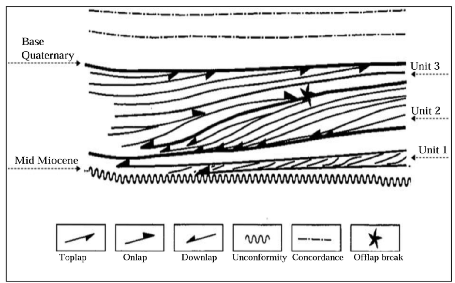
Figure 1: Sketch of the Neogene fluvio-deltaic...
Sketch of the Neogene fluvio-deltaic system in the Southern North Sea [25].
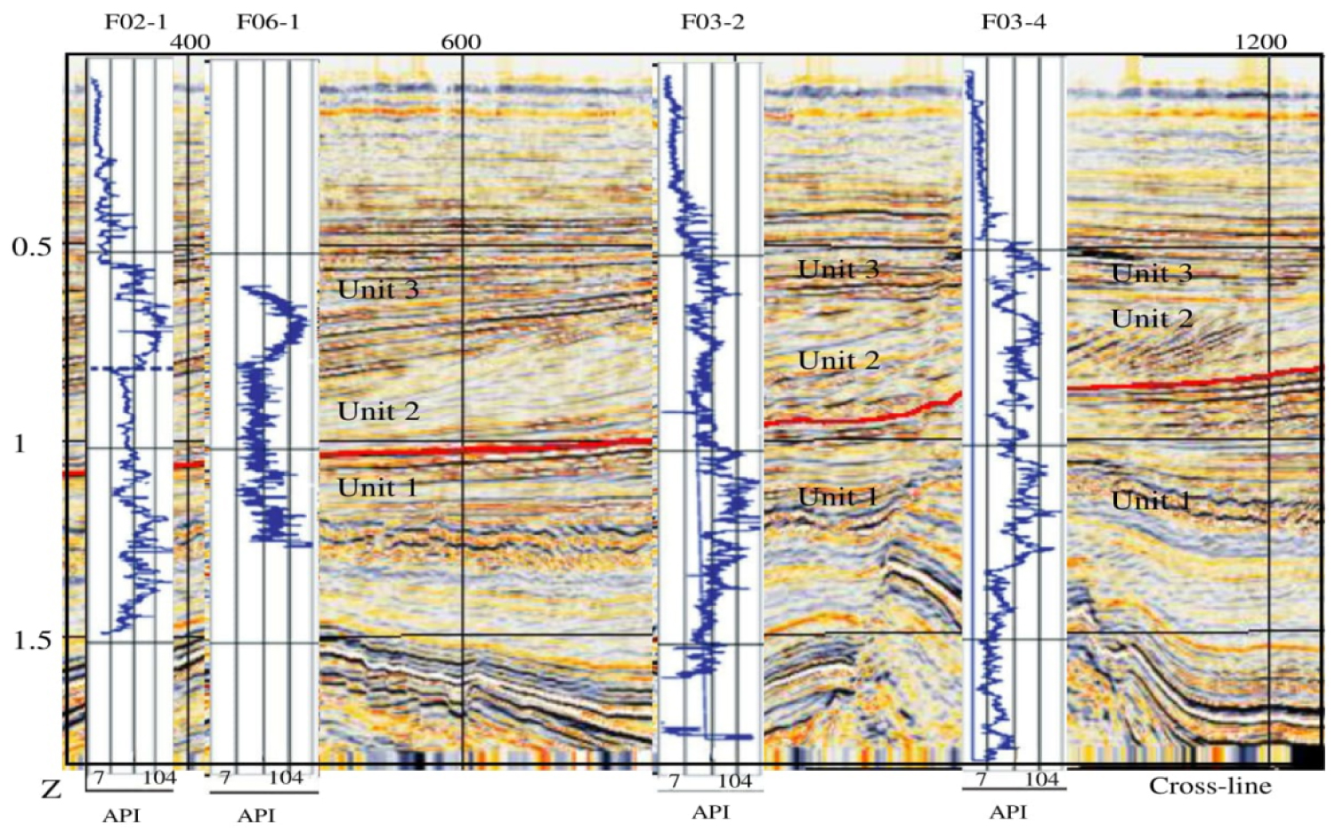
Figure 2: a) Relation between tuning thickness...
a) Relation between tuning thickness and frequency [31] and; b) Results of spectral decomposition at 36 Hz, 15 Hz, maps and channel thickness detected with variable frequency [41]. Low frequency slices indicate high thickness (green lines) and high frequency slices indicate low thickness (red lines).
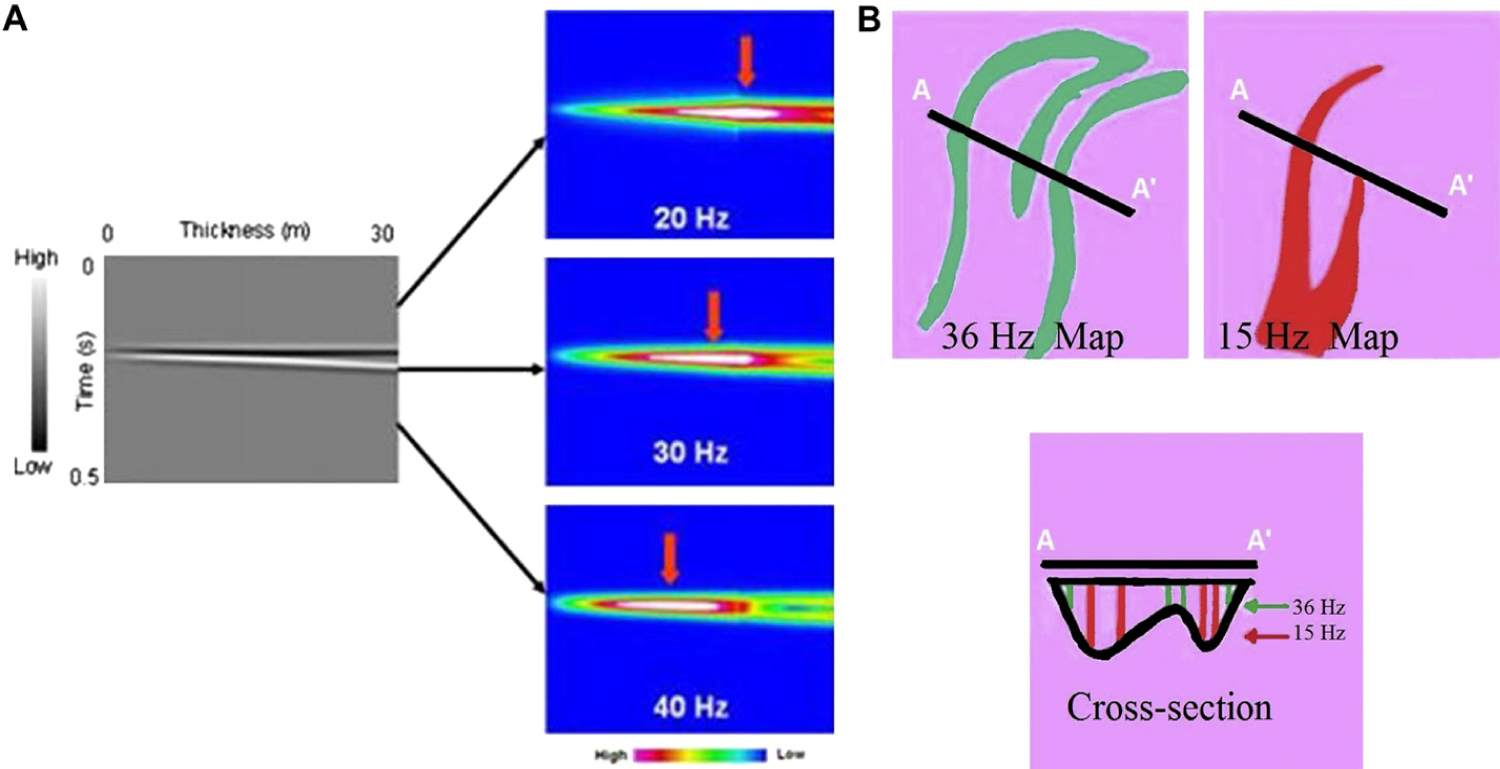
Figure 3: Vertical seismic section (inline 250)...
Vertical seismic section (inline 250) showing the mapped seismic horizon (red line) and the location of wells and the gamma ray logs of each well.

Figure 4: Time slices a) 1007 ms; b) 1028 ms;...
Time slices a) 1007 ms; b) 1028 ms; c) 1037 ms; d) 1055 ms; e) 1064 ms (red oval shape indicate the channel like feature. This feature is not delineated in time slice 1064 ms).

Figure 5: a) Display of inline 250 and the mapped...
a) Display of inline 250 and the mapped seismic horizon shown in red; b) Colour blended display of the mapped horizon shown in a; (c) Amplitude Spectrum of inline 250 showing the seismic bandwidth.

Figure 6: Comparison between the three mother...
Comparison between the three mother wavelets at 42 Hz frequency. The Gaussian wavelet gives better resolution of the channel features (indicated with red arrows) than the Morlet and the Mexican Hat wavelets.

Figure 7: Comparison between FFT and CWT a) 28 Hz...
Comparison between FFT and CWT a) 28 Hz FFT and; b) 28 Hz CWT; c) 42 Hz FFT and; d) 42 Hz CWT; e) 60 Hz FFT and; f) 60 Hz CWT.

Figure 8: (a) Stacked frequency volume of frequencies...
(a) Stacked frequency volume of frequencies 28 Hz, 42 Hz and 60 Hz; (b) RGB colour blending of frequencies 28 Hz (red), 42 Hz (green) and 60 Hz (Blue).

Figure 9: Display showing incised channels on...
Display showing incised channels on a coherence slice and its seismic amplitude signature. The seismic signature of the incised channel is seen as a sag at the position of the yellow arrows. We interpret the sag over the channels to indicate that they contain more shale than the surrounding matrix.

Figure 10: a) Coherence image; b) Most positive curvature...
a) Coherence image; b) Most positive curvature and; c) Most negative curvature, the yellow arrows delineate channel edges seen in the Coherence. Note that these channels can be followed further on the most negative curvature image. Notice the strong most-negative curvature anomaly along the channel axis (blue). We interpret the most negative curvature anomaly to be due to differential compaction over shale-filled channels.

Figure 11: a) Co-rendered coherence and most negative...
a) Co-rendered coherence and most negative curvature; b) Co-rendered most-positive and most-negative curvature volumes where moderate curvature values are rendered transparent. Sediments within the channel have undergone more compaction and give rise to a strong negative curvature anomaly along its axis (blue). Levees and channel edges appear as ridges and give rise to strong positive curvature anomalies (red).
References
- Evans DJ, Hopson PM, Kirby GA, Bristow CR (2003) The development and seismic expression of synsedimentary features within the chalk of southern England. Journal of the Geological Society 160: 797-813.
- Selvage J, Jones C, Edgar J (2012) Maximizing the value of 3D seismic data for shallow geohazard identification. First Break 30: 73-83.
- Bouanga E, Selvage J, Qayyum Q, Jones J, Brazier S, et al. (2014) Implications of horizoncubes in shallow hazards interpretation. First Break 32: 67-73.
- Schroot BM, Schüttenhelm RTE (2003) Expressions of shallow gas in the netherlands north sea. Geologie en Mijnbouw 82: 91-105.
- Stuart JY, Huuse M (2012) 3D seismic geomorphology of a large plio-pleistocene delta "bright spots" and contourites in the southern north sea. Marine and Petroleum Geology 38: 143-157.
- Qayyum F, Hemstra N, Singh R (2013) A modern approach to build 3D sequence stratigraphic framework. Oil and Gas Jourrnal 111: 46-65.
- Caldwell J, Chowdhury A, Engelmark F, Sonneland L, Neidell NS, et al. (1997) Exploring for stratigraphic traps. Oilfield Review 48-61.
- Tetyukhina D, Lucas J, Vliet V, Luthi SM, Wapenaar K (2010) High-resolution reservoir Characterization by an acoustic impedance inversion of a Tertiary deltaic clinoform system in the North Sea. Geophysics 75: 57-67.
- Marfurt KJ, Kirlin RL, Farmer SH, Bahorich MS (1998) 3D seismic attributes using a running window semblance-based algorithm. Geophysics 63: 1150-1165.
- Luo Y, Higgs WG, Kowalik WS (1996) Edge-detection and stratigraphic analysis using 3D seismic data. 66th Annual International Meeting, SEG Technical Program Expanded Abstracts, 324-327.
- Chopra S, Marfurt KJ (2006) Seismic attribute mapping of structure and stratigraphy. CSEG Recorder, Special Edition 110-121.
- Partyka GA, Gridley J, Lopez J (1999) Interpretational applications of spectral decomposition in reservoir characterization. The Leading Edge 18: 353-360.
- Marfurt KJ, Kirlin RL (2001) Narrow band Spectral analysis and thin bed tunning. Geophysics 66: 1274-1283.
- Castagna JP, Sun S, Seigfried RW (2003) Instantaneous spectral analysis: Detection of low frequency shadows associated with hydrocarbons. The Leading Edge 22: 120-127.
- Sinha S, Routh PS, Anno PD, Castagna JP (2005) Spectral decomposition of seismic data with continuous-wavelet transform. Geophysics 70: 19-25.
- Chakraborty A, Okaya D (1995) Frequency-time decomposition of seismic data using wavelet-based methods. Geophysics 60: 1906-1916.
- Leppard C, Eckersley A, Purves S (2010) Quantifying the temporal and spatial extent of depositional and structural elements in 3D seismic data using spectral decomposition and multi attribute RGB blending. Proceedings of the 30th Annual Bob F. Perkins Research Conference, Gulf Coast Section of SEPM Foundation, 1-7.
- Erlangga G, Afafa K, Sudarmaji M (2013) Colour blending on spectral decomposition method for delineating geological features. Proceedings of the Indonesian Petroleum Association, 37th Annual convention and Exhibition.
- Honório BCZ, Sanchetta AC, Leite EP, Vidal C (2014) Independent component spectral analysis. Interpretation, 21-29.
- Mojeddifar S, Kamali G, Ranjbar H (2015) Porosity prediction from seismic inversion of a similarity attribute based on a pseudo-forward equation (PFE): A case study from the North Sea Basin, Netherlands. Petroleum Science 12: 428-442.
- Sørensen JC, Gregersen U, Breiner M, Michelsen O (1997) High frequency sequence stratigraphy of upper cenozoic deposits in the central and southeastern North Sea areas. Marine and Petroleum Geology 14: 99-123.
- Ziegler PA (1990) Geological atlas of western and central Europe. (2nd edn), Shell International Petroleum Maatschappij 238.
- Overeem I, Weltje GJ, Bishop-Kay C, Kroonenberg SB (2001) The Late Cenozoic Eridanos delta system in the Southern North Sea Basin: A climate signal in sediment supply? Basin Research 13: 293-312.
- Rohrman M, Van der Breek P, Andriessen P, Cloetingh S (1995) Meso‐Cenozoic morphotectonic evolution of southern Norway: Neogene domal uplift inferred from apatite fission track thermochronology. Tectonics 14: 704-718.
- Sales JK (1992) Uplift and subsidence of northwestern europe: Possible causes and influence on hydrocarbon productivity.
- Ghazi SA (1992) Cenozoic uplift in the Stord Basin area and its consequences for exploration.
- Steeghs P, Overeem I, Tigrek S (2000) Seismic volume attribute analysis of the Cenozoic succession in the L08 block (Southern North Sea). Global Planetary Change 27: 245-262.
- Saadatinejad MR, Hassani H, Javaherian A (2011) Representation of the thickness distribution of channels and stratigraphic events at one of the Iranian field in the Hormuz strait using a composite plot and RGB display technique. Journal of Geophysics and Engineering 8: 412-421.
- Laughlin K, Garossino P, Partyka G (2002) Spectral decomposition applied to 3D. AAPG Explorer 23: 28-31.
- Chopra S, Marfurt K (2007) Seismic attributes for prospect identification and reservoir characterization. SEG Geophysical Development Series 11: 327-335.
- Lui J, Marfurt K (2006) Thin bed thickness prediction using peak instantaneous frequency. SEG Technical Program Expanded Abstracts 25: 51.
- Zabibi NE, Siahkoohi HR (2006) Single frequency seismic attribute based on short time fourier transform, continous wavelet transform, and S transform. 6th International Conference and Exposition on Petroleum Geophysics, Kolkata, 662-666.
- Morlet J, Arens G, Fourgeau E, Glard D (1982) Wave propagation and sampling theory-Part I: Complex signal and scattering in multilayered media. Geophysics 47: 203-221.
- Mallat S A (1999) Wavelet tour of signal processing. (2nd edn), Academic Press Inc.
- Chopra S, Marfurt K (2015) Is curvature overrated? No, it depends on the geology. First Break 33: 45-55.
- Aminzadeh F, de Groot PD (2006) Neural networks and other soft computing techniques with applications in the oil industry. Amsterdam: EAGE.
- Castagna JP, Sun S (2006) Comparison of spectral decomposition methods. First Break 24: 75-79.
- Mai HT, Marfurt KJ, Perez SC (2009) Coherence and volumetric curvatures and their spatial relationship to faults and folds, an example from Chicontepec basin, Mexico. SEG Houston, International Exposition and Annual meeting.
- Cao J, Yue Y, Zhang K, Yang J, Zhang X (2015) Subsurface channel detection using color blending of seismic attribute volumes. International Journal of Signal Processing, Image Processing and Pattern Recognition 8: 157-170.
- Torrado L, Mann P, Bhattacharya J (2014) Application of seismic attributes and spectral decomposition for reservoir characterization of a complex fluvial system: Case study of the Carbonera Formation, Llanos foreland basin, Colombia. Geophysics 79: 221-230.
- Chopra S, Marfurt K (2012) Seismic attribute expression of differential compaction. The Leading Edge 31: 1418-1422.
- Chopra S, Marfurt K (2007) Seismic curvature attributes for mapping faults/fractures, and other stratigraphic features. CSEG Recorder 32: 38-41.
- Chopra S, Marfurt K (2006) Curvature attribute applications to 3D surface seismic data. The Leading Edge 31: 404-414.
- Kwietniak A, Cichostepski K, Kasperska M (2016) Spectral decomposition using the CEEMD method, a case study from the carpathian foredeep. Acta Geophysica 64: 1525-1541.
- Luthi SM (2001) Geological well logs: Their use in Reservoir modelling. New York: Springer.
Author Details
Kenneth Samuel Okiongbo1* and Righteous Ombu2
1Department of Physics, Niger Delta University, Nigeria
2Department of Applied Sciences, Federal Polytechnic, Nigeria
Corresponding author
Kenneth Samuel Okiongbo, Geophysics Unit, Department of Physics, Niger Delta University, Wilberforce Island, Bayelsa State, Nigeria.
Accepted: April 04, 2019 | Published Online: April 06, 2019
Citation: Okiongbo KS, Ombu R (2019) Application of Spectral Decomposition and Seismic Attributes For Channel Geometry and Infill Lithology Determination: A Case Study from The Southern North Sea Basin. Int J Earth Sci Geophys 5:023.
Copyright: © 2019 Okiongbo KS, et al. This is an open-access article distributed under the terms of the Creative Commons Attribution License, which permits unrestricted use, distribution, and reproduction in any medium, provided the original author and source are credited.
Abstract
In the Southern North Sea, 3D seismic data had been widely acquired to explore for hydrocarbons, but interpretations of these datasets until now focus mainly on the deep exploration targets of the petroleum companies. Less attention is given to shallow sediments. But these sediments often contain channels that can serve as efficient stratigraphic traps for shallow gas. Thus the mapping and identification of these shallow channels and defining their infill lithology is important considering the abundance of shallow gas and its significance both as a ressource and hazard. In this study, seismic spectral decomposition technique has been used to delineate shallow thin channel geometry in a 3D seismic data acquired in the Dutch sector of the North Sea. The concurrent interpretation of curvature and coherence cubes with seismic facies analysis based on reflection terminations and geometry, amplitude and continuity enables the discrimination between shale versus sand filled channels. The results of the spectral decomposition show two distinct low sinuosity channel features in NNE-SSW direction but becomes diffuse towards the North. The strong negative curvature anomaly along the channels axes observed in the most negative curvature attribute implies that the sediments within the channels have undergone more compaction. These strong negative curvature anomalies are interpreted to be due to differential compaction of shale filled non productive channels.
Keywords
Spectral decomposition, Seismic, Lithology, North sea
Introduction
In the Southern North Sea, an extensive 3D seismic data had been acquired to explore for oil and gas in the Upper-Jurassic and Lower Cretaceous by the petroleum companies. But for most 3D seismic datasets, interpretations are focused mainly on the deep exploration targets of the petroleum companies. Less attention is given to shallow (younger) sediments. Presumably, this may be due to fact that these sediments are far above the main hydrocarbon findings on one hand, and on the other hand, their location too deep below the seabed for research by others than oil companies [1]. But these shallow (younger) sediments often contain channels that could serve as potential reservoir units cappable of trapping shallow gas. The mapping and identification of these shallow channels and defining their infill lithology in a fluvio-deltaic system is thus important in exploration and production. This is because these channels could serve as tools for shallow geohazard analysis [2,3]. For instance, in a gas filled shallow stratigraphic trap, the gas can be a hazard and a risk when drilling a borehole [4-6]. Additionally, the occurrence of a shallow gas filled stratigraphic trap can be an indication for the presence of deeper hydrocarbon reserves, and thus an exploration tool. Besides, some of the shallow gas fields are even big enough to be considered as commercial gas fields [5].
Channels are generally visually close to or below seismic resolution [7,8], so thin to their surrounding geometry that their subtleties are nearly invisible in traditional seismic data. Thus, delineating thin reservoir sands from conventional seismic data had always been a challenge. Recent innovations such as coherence technology [9] and other edge sensitive attributes [10] are common methods employed in mapping boundaries of these geological subtle targets (channels). Although coherence images and edge sensitive attributes reveal channels edges, a key limitation in these techniques is that they cannot delineate the channel's thickness [11].
Spectral decomposition is a recent seismic interpretation technology that reveals otherwise hidden geological information and thus is being used extensively as an excellent tool for mapping channels [12]. In spectral decomposition, reflection from a thin bed has a peculiar expression in the frequency domain that gives an indication of the temporal bed thickness. It is a powerful seismic imaging and mapping tool that provides the interpreter useful quantitative information for determining bed thickness [12], visualization of stratigraphy [13] and detection of hydrocarbon [14,15] to a level that was previously impossible. Spectral decomposition is also an effective tool in enhancing geohazard analysis as it is sensitive to wavelet, reflectivity, tuning and attenuation changes [2]. In spectral decomposition, the seismic data is converted from the time domain to the frequency domain and decomposed into frequency components. Studying the individual frequency components and comparing their responses provides significant insight into the subsurface geology. The time-frequency mapping process is a non-unique process; as a result, there are several methods for carrying out time-frequency analysis of non-stationary signals. Popularly used spectral decomposition methods include Fast Fourier Transform (FFT), Continuous Wavelet Transform (CWT), S-transform (ST), and Matching Pursuit decomposition (MPD). It is important to note that each method has its strengths and weaknesses [16,17].
Several published works have discussed thoroughly various aspects of the post-stack time migrated 3D seismic dataset provided by dGB Earth Sciences in the F3 block. Some of these studies carried out in the study area are on delineation of geological features using spectral decomposition [18], independent spectral analysis [19], porosity prediction from seismic inversion [20] etc. Although these studies and others provide very rich literature on various aspects of the dataset, studies on prediction of the infill lithology of fluvio-deltaic channels particularly in the shallow (younger) sediments distinguishing channels filled with sand from those filled with shale are lacking. In this study, we have used attribute-assisted interpretation workflow to study the shallow channel geometry and infill lithology. We have applied FFT and CWT methods of spectral decomposition and seismic attributes (coherence and curvature) to a 3D seismic data set acquired in the upper Cenozoic fluvio-deltaic system in the block F3 in the North Sea basin to delineate shallow thin channel geometry and distinguish between intrachannel shale versus sand lithologies. The intrachannel lithologies predicted using the seismic attributes were validated using well logs available in the area in conjunction with other lines of evidence.
Geological setting
The study area (F3 block) is located in the Dutch sector of the North Sea. Much of the entire North Sea region in the Cenozoic era was a thermally subsiding epicontinental basin that was confined by land masses [21]. Sedimentation rates during the Neogene outpaced the subsidence rate, resulting in rapid deposition and shallowing of the North Sea basin. An extensive fluvio-deltaic system (Eridanos delta) prevailed in the basin during the late Cenozoic Period [22, 23], draining the Fennoscandian High and the Baltic Shield. According to Overeem, et al. [23], the Eridanos drainage developed due to the Neogene uplift of the Fennoscandian Shield and accelerated subsidence of the North Sea Basin that occurred at the same time. The drainage system (Eridanos delta) started when the Scandinavian Shield was uplifted during the Oligocene [24].
Sales [25] reported that the uplift rate increased during the late Miocene and also in the early Pliocene [26]. Due to the late Miocene uplift, high sediment influx filled the northern offshore regions of the Dutch Sector. The increasing sediment load resulted in a differential load throughout the region. As a result, the buried Permian Zechstein salt started moving in the region forming several localized unconformities within the Pliocene interval that are underlain by salt domes.
The Cenozoic succession consists of two main packages, separated by the Mid-Miocene Unconformity [27] (Figure 1). The lower package consists predominantly of relative fine-grained gradational Paleogene sediments [27], while the package above the unconformity is largely a progradational deltaic sequence that are made up of coarse Neogene sediments. The package above the unconformity can be subdivided into three sequences (Units 1, 2, and 3) corresponding to three phases of delta evolution (Figure 1). Generally, in this package, conspicuous large-scale sigmoidal bedding pattern, downlap, toplap, onlap and truncation structures are observed. The base of Unit 2 is the zone of interest for this study. Unit 2 is the delta forest with a coarsening upward sequence [23] and the age of this unit is estimated to be Early Pliocene.
Theoretical foundation
Spectral decomposition methods
The thin-bed tuning effect is the reason for the application of spectral decomposition method on a seismic data. The thin-bed tuning effect occurs when reflections from top and down layers have a constructive interference. In this instance, the peak amplitude response will occur at ¼ wavelength of the dominant period and layer thickness less than this value will not be detected in the seismic section [28]. Laughlin, et al. [29] illustrated the relationship between tuning thickness and frequency using a wedge synthetic seismic model (Figure 2). Figure 2a shows a thickness increase from 0 to 30 m at the left side, while the right side indicates amplitude tuning in three different frequencies. Figure 2b shows the basis of the spectral decomposition technique, high frequency (36 Hz, green colour) delineates the thinner part of the paleo channel and the low frequency (15 Hz, red colour) shows the thicker part [30,31].
Fast Fourier Transform (FFT)
The Fourier transform of a time-domain seismogram is expressed mathematically as:
Where t is time. Although a non-stationary signal when converted into the frequency domain via the Fourier transform method gives the overall frequency behaviour of the signal; such a transformation is not adequate for analysing seismic data (a non-stationary signal), whose frequency content is not constant but varies with time. By taking short segments of the signal which are considered stationary parts (i.e., windowing the signal) and then performing the Fourier transform for each segment, provides the frequency content of the signal at that time period [16,32]. When this time window is shifted appropriately, it is possible to extract the frequency content of the signal and thus produce a 2-D representation of frequencies versus time. This 2-D representation is commonly known as short-time Fourier transform (STFT). The implementation of FFT is based on Short Window Discrete/Fast Fourier Transform.
The STFT is given by the inner product of the signal with a time-shifted window function expressed mathematically as:
Where the window function is centered at time , with being the translation parameter, and is the complex conjugate of .
Continuous Wavelet Transform (CWT)
The continuous wavelet transform (CWT) introduced by Morlet, et al. [33] is another method used to analyze the time-frequency content of a signal. Unlike the STFT where the window function has a fixed length, the CWT uses a variable window length. If the length of the interval on which the window function is non zero increases, the time resolution decreases, and the frequency resolution increases. On the other hand, when the length of the interval decreases, the time resolution increases and the frequency resolution decreases. The foregoing means that by increasing the frequency resolution, the time resolution will decrease and vice versa [34].
The wavelet transform consists of wavelets which are functions defined as that have zero mean, which is localized in both time and frequency [15]. Each wavelet basis is generated by dilating and translating a two parameter function known as the mother wavelet, . Given a wavelet basis, we can represent all functions in the basis by translations and scalings of the mother wavelet,
Where and are the dilation or scale and translation parameters. In Eq. 3, as the value of increases, the wavelet is compressed, its spectrum dilates and the peak frequency shifts to a higher value. Conversely, as the wavelet is scaled such that it dilates, the value of decreases, its spectrum is compressed and the peak frequency shifts to a lower value [35]. The CWT is defined as the inner product of the family of wavelets with the signal given as:
Where the complex is conjugate of and is the time-scale map (scalogram). At each scale (i.e., for each value of ) the kernel wavelet is scaled by a factor 1/ and translated by to produce the wavelet coefficients . Useful wavelets commonly used in wavelet transform are Morlet, Gaussian and Mexicat-Hat.
Materials and Method
The dataset used in this study is a post-stack time migrated open source 3D seismic dataset that was acquired in the F3 block covering an area of approximately 16 × 23 km2 to explore for oil and gas in the Upper Jurassic and Lower Cretaceous made publicly available by dGB Earth Sciences through OpendTect share seismic data repository [36]. The F3 is a block located in the North-eastern part of the Dutch sector of the North Sea. The 3D seismic data is made up of 650 inlines and 950 crosslines with a line spacing of 25 m in both inline and crossline direction. The sampling rate is 4 ms with a total data length of about 1.8 s. Figure 3 shows a vertical seismic section (in line 250) with gamma ray logs overlaid on the section in the respective well locations (F02-1, F06-1, F03-2 and F03-4). The study area is the horizon (in red) at the base of Unit 2 located between 800 ms and 1100 ms (Figure 3). Because the original F3 dataset is noisy, only Dip-steered Median Filtered dataset was used as input data in this study.
Since this study is aimed at delineating channels and to distinguish between sand-fill from shale-fill channel system in the study area, time slices of the 3D seismic volume was carried out between 1000 ms and 1055 ms, and the geological features in each time slice was analysed. In time slice 1007 ms (Figure 4a), a channel like feature having a NNE-SSW pattern was observed, and extended towards the southern part in time slices 1028, 1037 and 1055 ms respectively (Figure 4b, Figure 4c and Figure 4d). At time slice 1055 ms, only a small part of the feature was observed and become indiscernible in time slice 1064 ms (Figure 4d). From the above, it implies that a channel system existed between 1007 and 1055 ms which shows maximum prominence at 1028 and 1036 ms. Based on this, the horizon shown in red was picked for analysis (Figure 5a and Figure 5b).
We also analysed the amplitude spectrum of the data (Figure 5c). We define three dominant frequencies from the amplitude spectrum for RGB multi-colour display. The three frequencies were chosen such that they represent the low (28 Hz), middle (42 Hz) and high (60 Hz) frequency of the seismic bandwidth around the horizon. The three frequencies were then output as a single RGB blended full colour image. This is important because mixing outputs of different frequencies enables us to analyse results that depict different geological features related to different geometrical scales simultaneously i.e., higher frequencies reveal features of more detailed character, whereas lower frequencies those which are more coarse. In using the CWT technique for spectral decomposition, the choice of the wavelet is important as it affects the output result [35,37]. As a result, we tested all three mother wavelets i.e., Morlet, Gaussian and Mexican-Hat wavelets to determine which wavelet would give better resolution. Figure 6 shows comparison of the resolution of the channel features of the three mother wavelets at 42 Hz frequency.
Although the resolution of the Mexicat-Hat and Gaussian mother wavelets appears to be similar (Figure 6), the Gaussian wavelet resolution of the channel features is slightly superior to that of the Mexican-Hat wavelet. Hence the Gaussian wavelet was chosen as the ideal mother wavelet for this data. In carrying out the spectral decomposition, we applied the low, middle and high frequencies on both the FFT and CWT (Figure 7).
In the spectral images shown in Figure 7, we observed that some parts of the channel are resolved better at low frequency, some at mid frequency and others at higher frequency. However, at 42 Hz frequency, a clearer image of the channel is observed. This frequency at which the channel geometry is clearly pronounced is the tuning frequency. Since different parts of the channel features are resolved at different frequencies, it was considered that the channel geometry can be obtained in its complete form when the different frequencies are stacked together. Thus, a stacked frequency volume was obtained by summing up the 28 Hz frequency (low frequency), 42 Hz frequency (mid frequency) and 60 Hz frequency (high frequency) volumes (Figure 8a). We used RGB colour-blending technique to display the multiple spectral components in a single 'full colour' image. Figure 8b displays RGB colour blending of the frequencies 28 Hz (red), 42 Hz (green) and 60 Hz (blue). In addition to FFT and CWT, we also generated coherence attribute image. The coherence attribute also known as similarity is an effective tool in determining lateral changes in the waveform and enables the mapping of lateral changes that might occur in stratigraphy [38].
Sandstones and claystones are the main infill rock types of paleo channels [39]. Each of these lithotypes has different responses to compaction, hence the lateral changes that accompany compaction of a rock volume as it lithifies in a channel depends on the type of lithology [40,41]. Because shales compact faster than sand [40], a channel filled with sand and suspended in a shaly matrix may look like a mound or 'structural' high while a channel that is filled with shale in a sandier interfluve may appear as structural low [41-43]. Such patterns are exploited as lithologic indicator. Since coherence and curvature attributes are sensitive to tectonic deformation including incisement and differential compaction of stratigraphic horizons [35], we have used the coherence and curvature attributes in a complementary manner through co-rendering to discriminate shale versus sand lithologies based on differential compaction of the channels relative to their edges. In this approach, coherence attribute was used to enhance the channel edges, the most post-positive curvature attribute was used to delineate likely levees and flanks of the channels (red) while the most - negative curvature attribute delineates the edges of the channel (blue) [40-43].
Results and Discussion
Results of the spectral decomposition comparing between FFT and CWT algorithms are shown in Figure 7. The comparison is to enable verify potential differences between the methods. In Figure 7, two significant distinct channel features are observed, particularly by the frequency of 42 Hz and are shown using red circles. The general direction of the channels observed is NNE-SSW and exhibit low sinuosity. Though the channels shape and low sinuosity are revealed by both algorithms, the CWT algorithm enhances the channel features better, the FFT results were considered rather poor. We attribute this behaviour to the length of the time window used for the FFT decomposition process. This is because the length of the time window used for the FFT decomposition is of paramount importance and the output of the FFT decomposition is always dependent on this characteristic [44].
In using different frequencies, features of different scales are separated. High frequencies delineate smaller features, whereas low frequencies delineate more coarse structures. This effect is visible by comparing Figure 7a, Figure 7b and Figure 7c. Figure 7d, in its left southern part, there is a more pronounced sign of the channel continuity (indicated with red circle) that was barely visible with lower frequencies especially with the FFT algorithm. We believe that the channel's width and thickness are smaller in this part than those which are visible for lower frequencies. Additionally, the channel on the right (Figure 7e and Figure 7f) appears to have a branch towards the southern part (indicated with a red circle). This feature was not observed in the FFT algorithm and was barely visible even in the CWT at lower frequencies, but become pronounced at higher frequencies. This suggests that the main channel is relatively thicker than its branch. This otherwise hidden geological information is important both for prospect evaluation and for quantifying reservoir heterogeneity.
Mixing outputs of different frequencies enables us to analyse results that depict different geological features related to different geometrical scales simultaneously i.e., higher frequencies reveal features of more detailed character, whereas lower frequencies reveal those which are more coarse. Figure 8 shows a RGB colour blended full colour image using 28 Hz (in red), 42 Hz (in green) and 60 Hz (in blue). The RGB colour blending also distinctly depicts the channel configuration mentioned above. The intensity of each primary colour represents the intensity of the attribute in that channel.
Figure 9 shows a coherence attribute image showing the channel features through a seismic section perpendicular to the thalweg of the channels. We have also used the coherence attribute to enhance channel edges (Figure 10a). Figure 10b and Figure 10c show the most-positive and the most-negative curvature volumes computed from the picked horizon.
Spectral decomposition analysis is an important reservoir imaging tool that helps in delineating subtle geological features such as channels. In this study, the Fast Fourier Transform (FFT) and Continuous Wavelet Transform (CWT) are used in delineating these geological features in the F3 block in the North Sea. The results show two distinct channel features that are significant in terms of hydrocarbon exploration and production. This is because nonproductive (shale filled) and productive (sand filled) channels exhibit similar seismic character [40]. In the coherence attribute image (Figure 9), we observed a sag. The sag observed in the vertical seismic section (yellow arrows) in Figure 9 indicates differential compaction and corresponds to the incised channels in the coherence image, consistent with the observation of Chopra and Marfurt [41] and Torrado, et al. [40], who reported that differential compaction can also be seen in seismic amplitude section. The most-positive curvature in Figure 10b delineates the likely levees and flanks of the channels, while the most-negative curvature indicates the channel axis (thalwegs) [41]. Figure 10C shows a strong negative curvature anomaly along the channel axis (blue), implying that sediments within the channels have undergone more compaction. In the coherence image shown in Figure 10a, the channels become progressively thinner towards the North, eventually fall below tuning and become indistinct. Co-rendering (i.e., simultaneously displaying) coherence and the most negative curvature (Figure 11a) shows how the curvature and coherence attributes can be used in a complimentary manner, in that in the lower part of the Figure where the channels are relatively thick, the coherence edges and channel axises mimic each other. That is, the curvature anomalies correlate to the channel geometry delineated in the coherence image and one can trace the channel geometry further on the most-negative curvature image even though the coherence channel edge anomalies become diffuse or disappear towards the North. Figure 11b shows co-rendered most-positive (red) and most-negative curvature (blue). Figure 11 shows a strong negative curvature anomaly along its axis (blue). This implies that sediments within the channel have undergone more compaction [40,41]. These strong negative curvature anomalies are interpreted to be due to differential compaction of shale filled non productive channel. Levees and channel edges are delineated as mounds or ridges and give rise to strong positive curvature anomalies (red).
In order to validate our prediction of the infill lithology, we overlay the gamma ray logs of the respective wells on the seismic section (Figure 2) with the horizon of interest shown in red. This horizon is at the bottom of Unit 2. According to Figure 2, the horizon of interest is at an interval rich in sediments with gamma ray values generally greater than 70 API [45]. This is consistent with the observation of Tetyukhina, et al. [8] who reported that shaly sediments with higher impedance values were deposited mainly at the bottomset of the clinoform system in the F3 block of the Southern North Sea basin.
Conclusion
The delineation of subtle geological features such as channels has always been a challenge. This is because channels are subseismic, so thin to their surrounding geometry that their subtleties are nearly invisible in traditional seismic data. But these geobodies are important because they serve as hydrocarbon traps. In an attempt to delineate shallow thin sand reservoirs in the F3 block, we have carried out spectral decomposition analysis using the Fast Fourier Transform (FFT) and Continuous Wavelet Transform (CWT) on a 3D seismic data acquired in the F3 block. We assessed the relative performance of the FFT and CWT on the data. We used a red-green-blue (RGB) colour-blending technique to display the composite full colour image to enhance better resolution of the channels features. In order to determine the infill lithology of these channels, we have also used the coherence and curvature attributes in a complementary manner. While the coherence attribute was used to enhance channel edges, the curvature attribute was used to discriminate between intrachannel shale versus sand lithologies based on differential compaction of the channel relative to its edges.
The results show two distinct almost linear channels trending in the NNE-SSW direction. The CWT algorithm remarkably delineated the channel geometries in a much better way than the FFT algorithm. While the most positive curvature defines the likely levees and overbank deposits and as well as the flanks of the channel, the most negative curvature defines the channel axis. The curvature anomalies also correlate to the channels geometry obtained from the coherence attribute. The strong negative curvature along the axis of the channel is due to differential compaction of a channel filled likely with shale.
Acknowledgments
The authors are extremely grateful to Danvic Concepts International Ltd, who collaborated with Nigerian Agip Oil company to promote geoscience training in Nigerian Universities. We are also grateful to dGB Earth Sciences for making the seismic data freely available for the public and for providing the OpendTect software for academic research.