
International Journal of Earth Science and Geophysics
(ISSN: 2631-5033)
Volume 6, Issue 1
Research Article
DOI: 10.35840/2631-5033/1833

Article Formats
Spatial-Temporal Analysis and Short-Term Forecasting of Hydrotechnical Facility Displacements
Table of Content
Figures
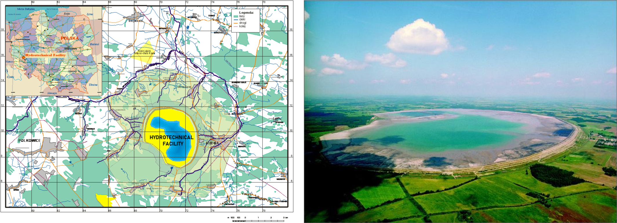
Figure 1: Location and general view of the foreground....
Location and general view of the foreground and the crown of the analyzed hydrotechnical object.
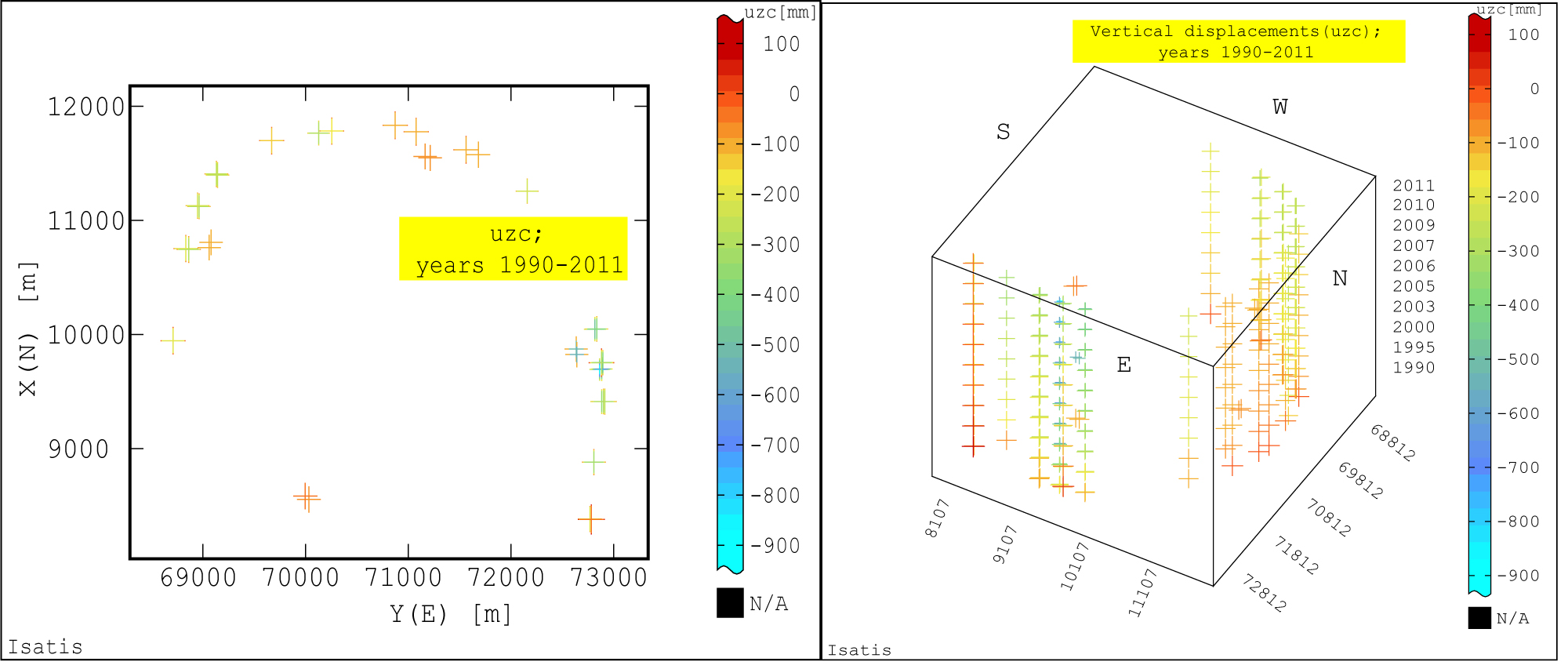
Figure 2: Base Map (a) and Base Map (in perspective).....
Base Map (a) and Base Map (in perspective) (b) of distribution of vertical displacements (uzc) of the benchmarks (BMs) in the dams of hydrotechnical facility (time database: Years 1990 ÷ 2011).
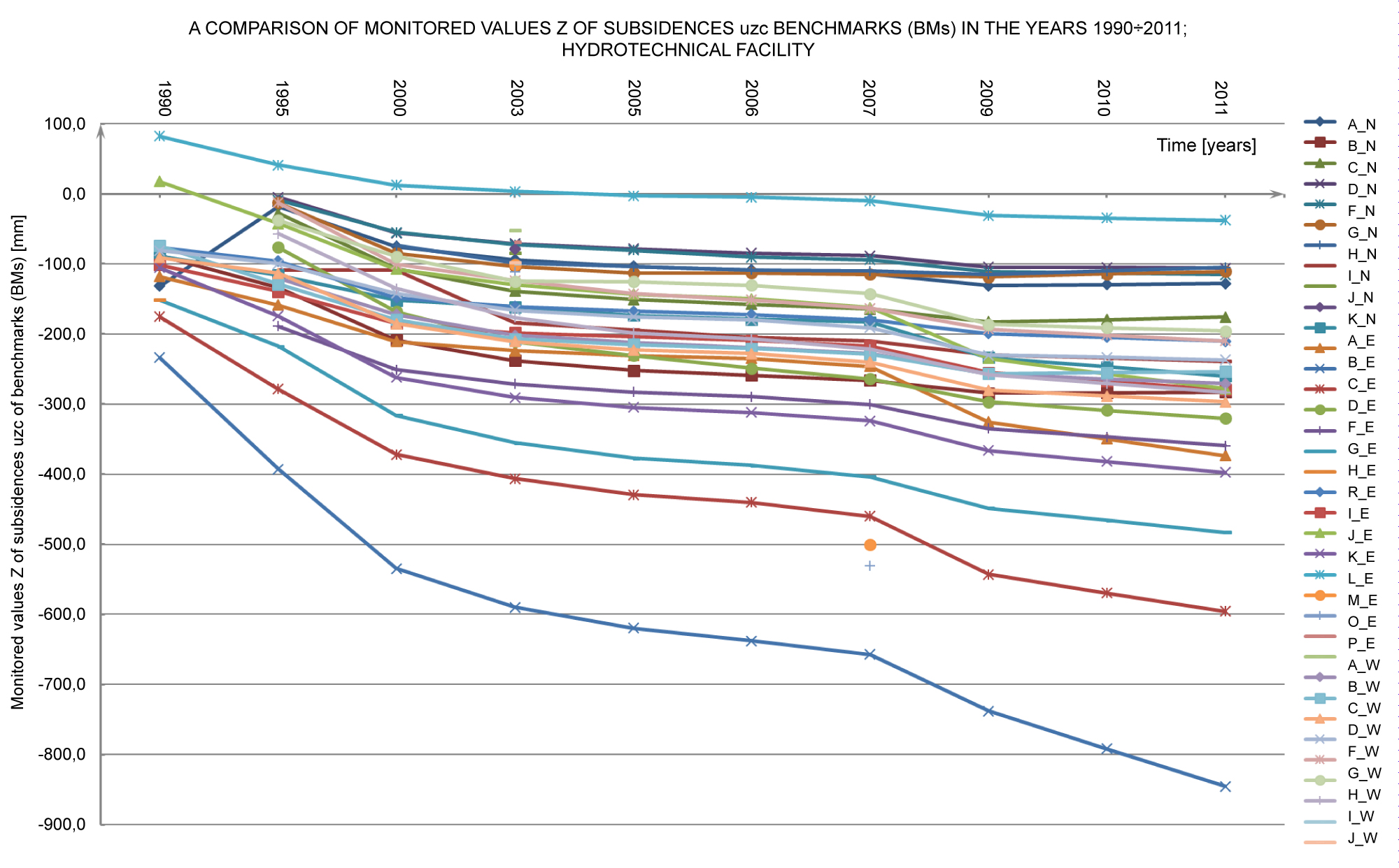
Figure 3: A comparison (plot) of monitored subsidences....
A comparison (plot) of monitored subsidences values Z of the BMs on the dams N (northern), E (eastern), S (southern), W (western) of hydrotechnical facility, in the years 1990 ÷ 2011.
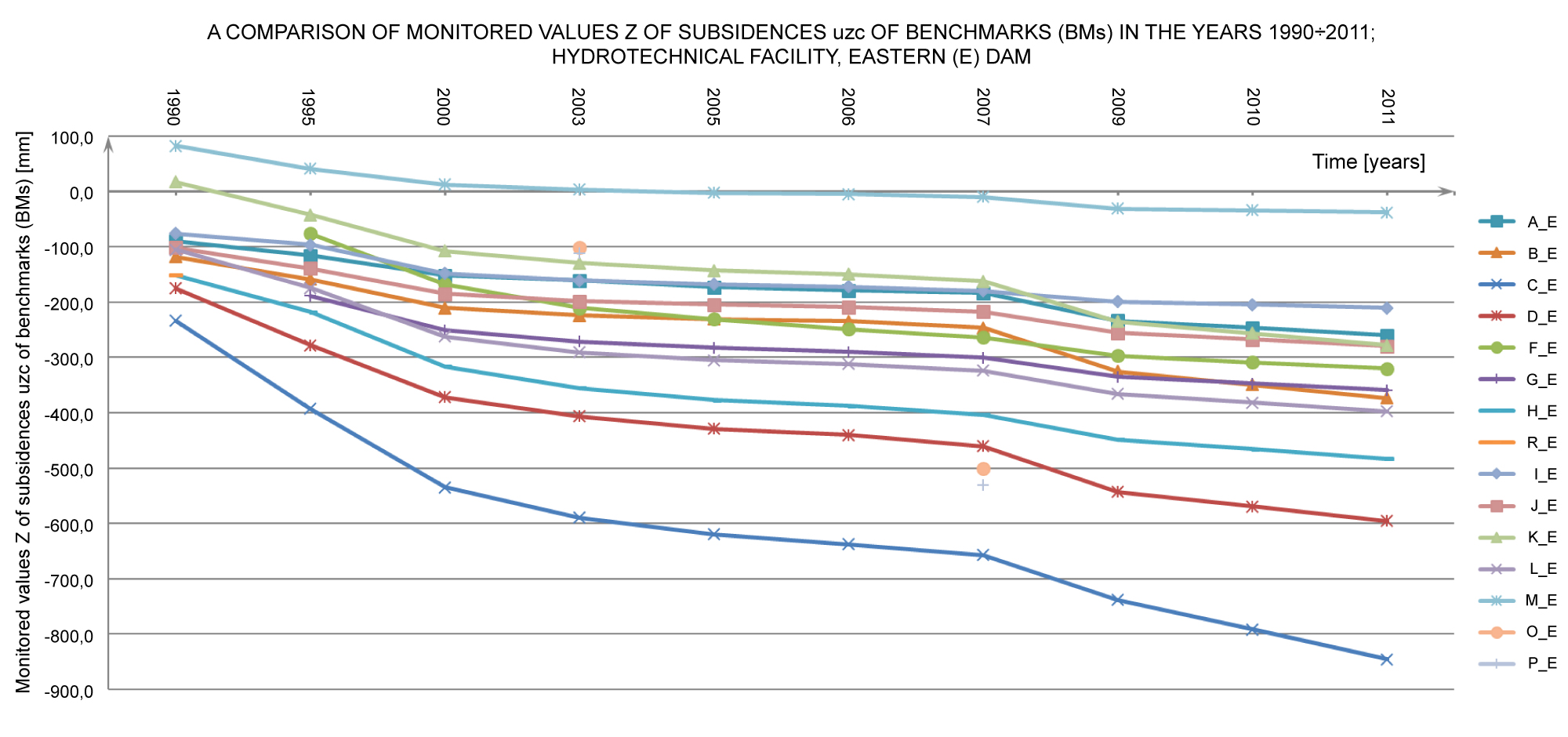
Figure 4: A comparison (plot) of subsidences values....
A comparison (plot) of subsidences values uzc of the BMs on the E (eastern) dam of hydrotechnical facility, in the years 1990 ÷ 2011.
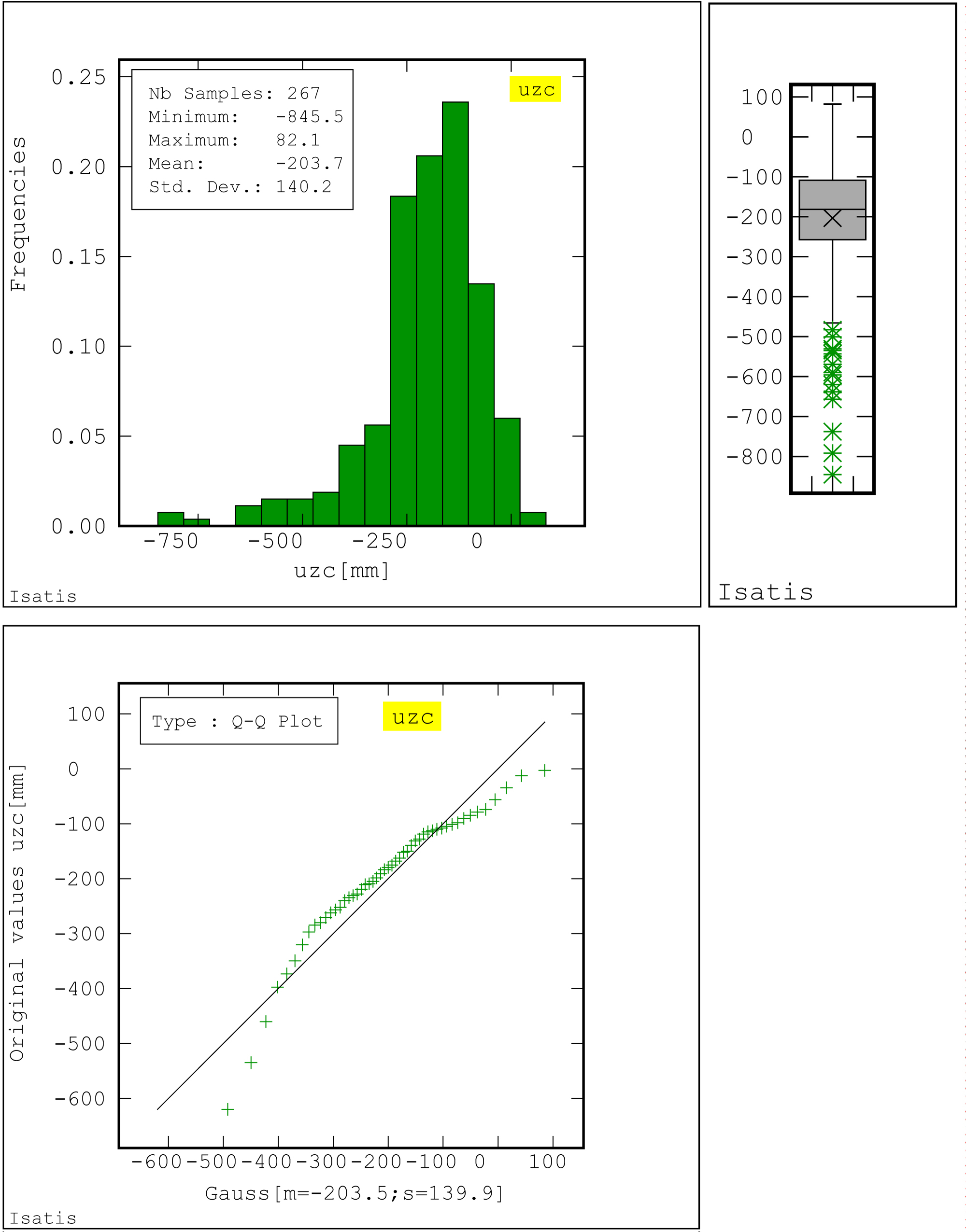
Figure 5: Histogram of distribution of vertical distribution....
Histogram of distribution of vertical displacements uzc in the dams of hydrotechnical object (skewness coefficient g1= -1.52; kurtosis coefficient g2 = 6.53 ; Quantiles: Q25 = -257.35, Q50 = -181.60, Q75 = -108.75) (a); Boxplot of displacements; time database: years 1990 ÷ 2011 (b); Q-Q Plot Quantile - quantile plot, Comparing the experimental distribution with the Gaussian distribution (c).
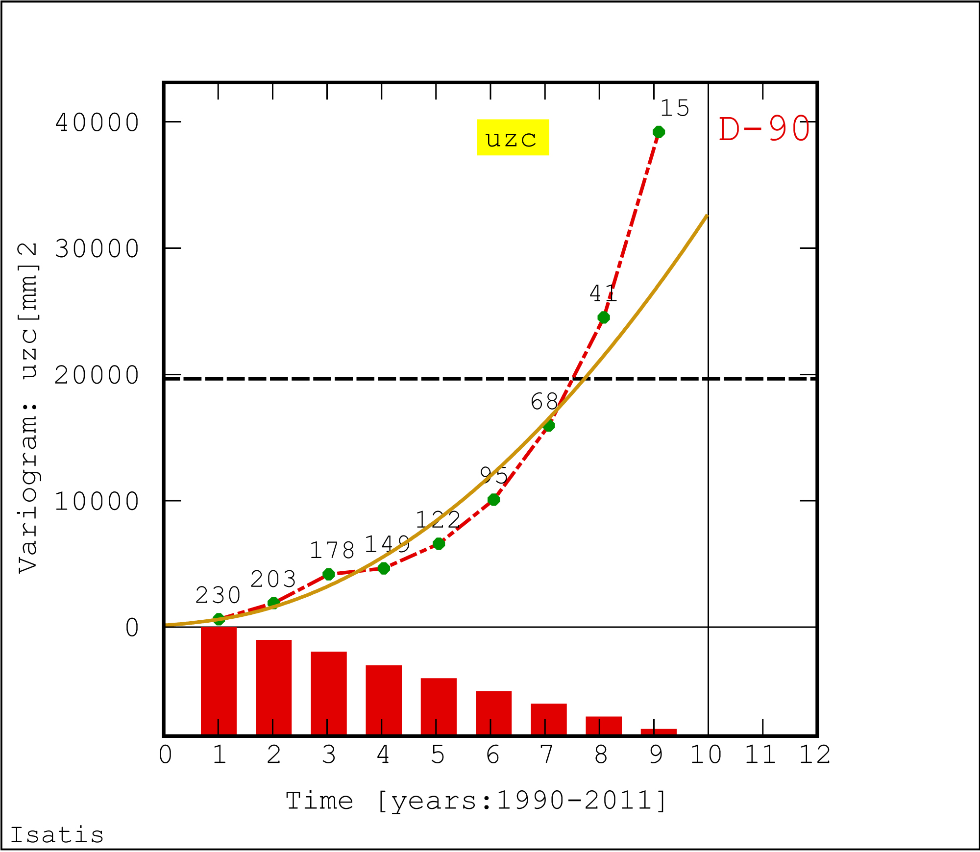
Figure 6: Directional semivariogram (D-90) of vertical displacements....
Directional semivariogram (D-90) of vertical displacements uzc of the BMs in the hydrotechnical facility, with the fitted theoretical model (along the time axis; years: 1990 ÷ 2011); green points in the graph - number of pairs; histogram of number of pairs.

Figure 7: The results of the cross-validation procedure for...
The results of the cross-validation procedure for the assumed theoretical model of directional semivariogram of vertical displacements uzc for BMs, years: 1990 ÷ 2011; the errors of assessments in the points (BMs) for the hydrotechnical facility, using the moving "kriging" neighborhood; the graph of the dependence of the actual (true) values of Z and estimated averages values Z* - correlation coefficient value r (a); The base map of the original values of vertical displacements uzc (b); The histogram of standardized error values distribution (Z* - Z)/S* (c); Graph of dependence of standardized error values (Z* - Z)/S* and estimated averages Z* (d).

Figure 8: Elementary grid (3D), used during estimating of...
Elementary grid (3D), used during estimating of vertical displacements uzc for subsoil of hydrotechnical object in the XOY, XOZ, and YOZ planes; time database of displacements uzc years 1990 ÷ 2011.
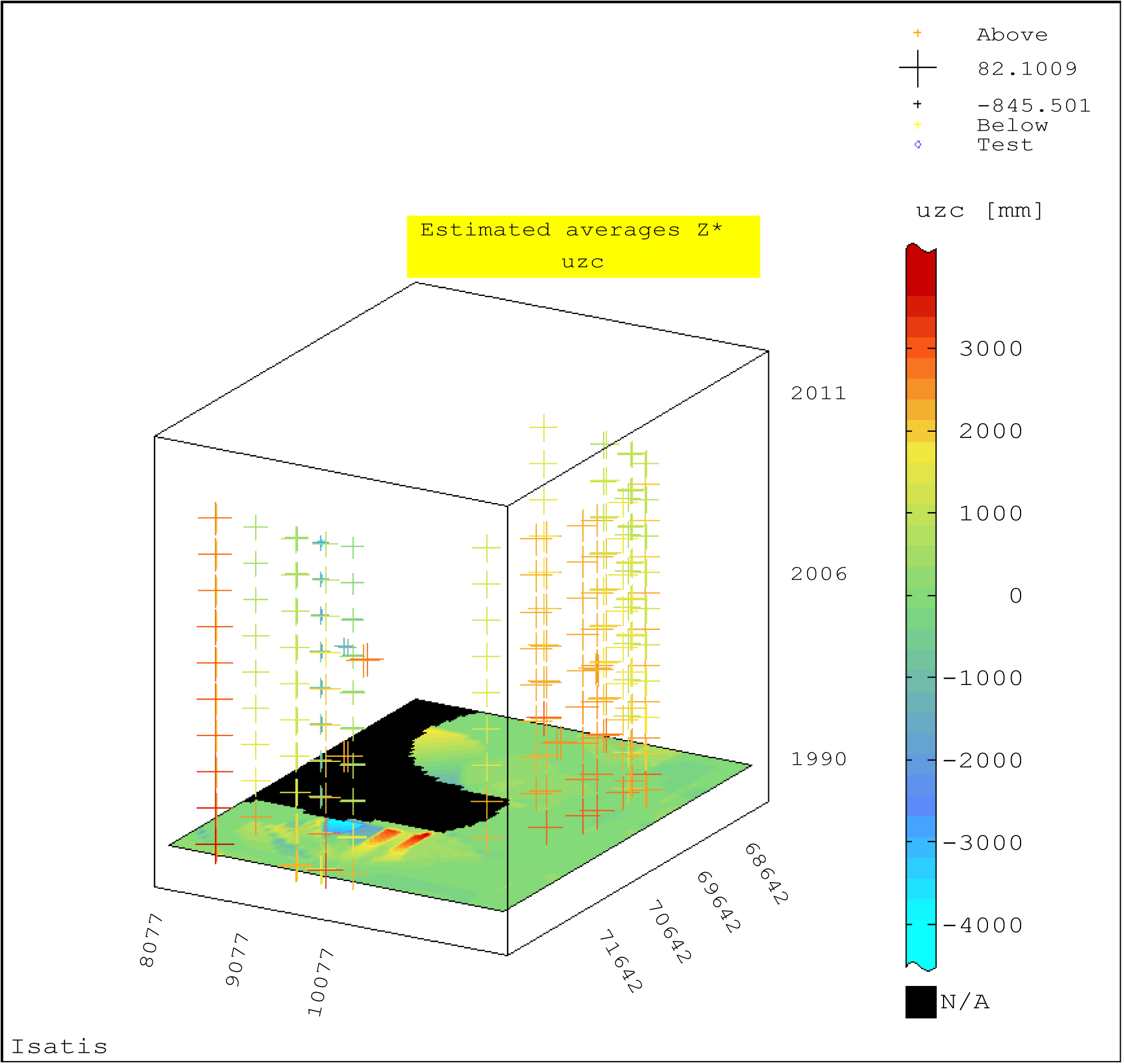
Figure 9: Block-diagram of estimated values Z* of vertical...
Block-diagram of estimated values Z* of vertical displacements uzc of the BMs in the hydrotechnical + facility (year 1990); ordinary (block) kriging; moving kriging neighborhood.

Figure 10: Block-diagram of estimated values Z* of vertical...
Block-diagram of estimated values Z* of vertical displacements uzc of the BMs in the hydrotechnical facility (year 2005); ordinary (block) kriging; moving kriging neighborhood.
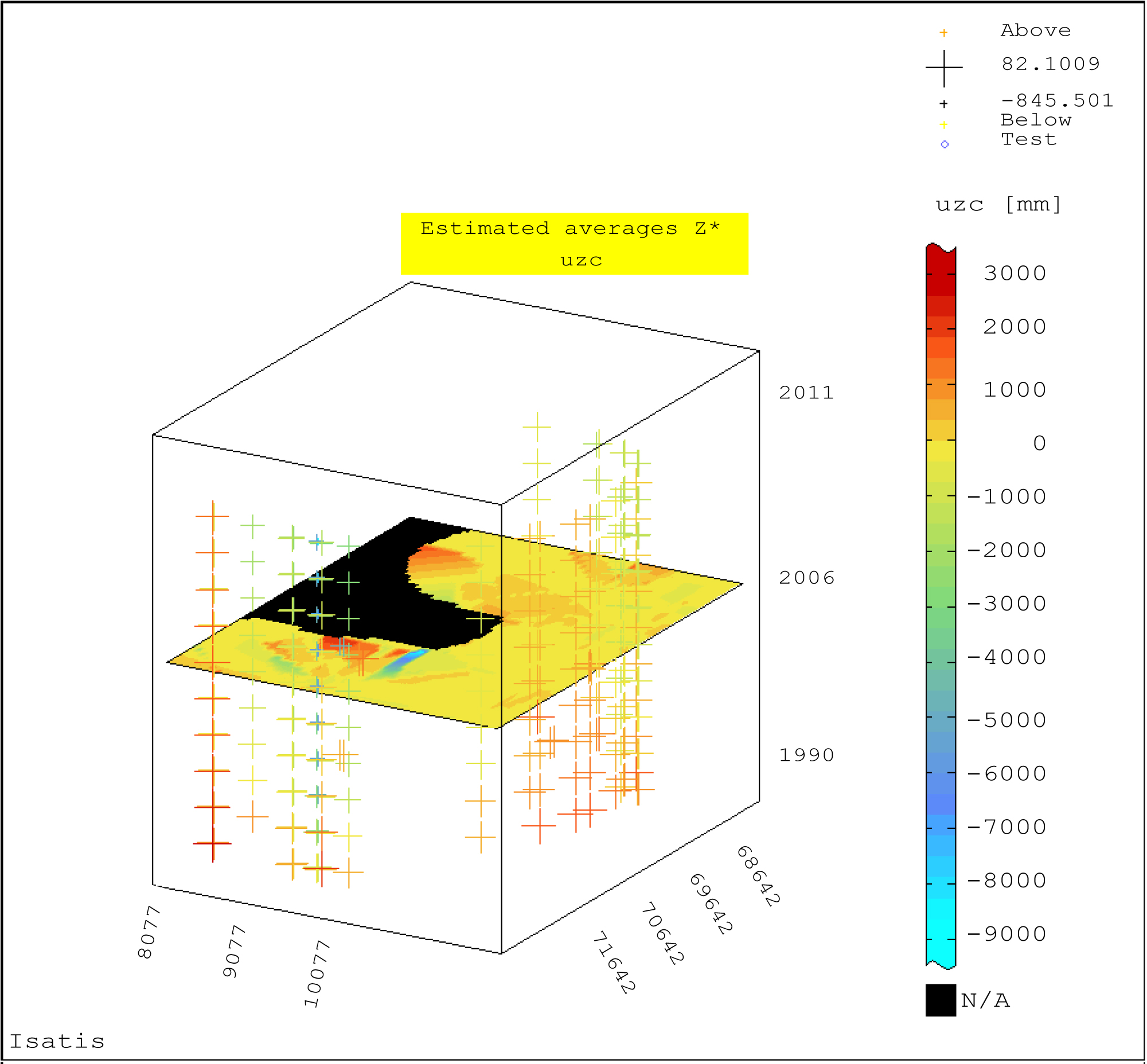
Figure 11: Block-diagram of estimated values Z* of vertical...
Block-diagram of estimated values Z* of vertical displacements uzc of BMs in the hydrotechnical facility (year 2006); ordinary (block) kriging; moving kriging neighborhood.
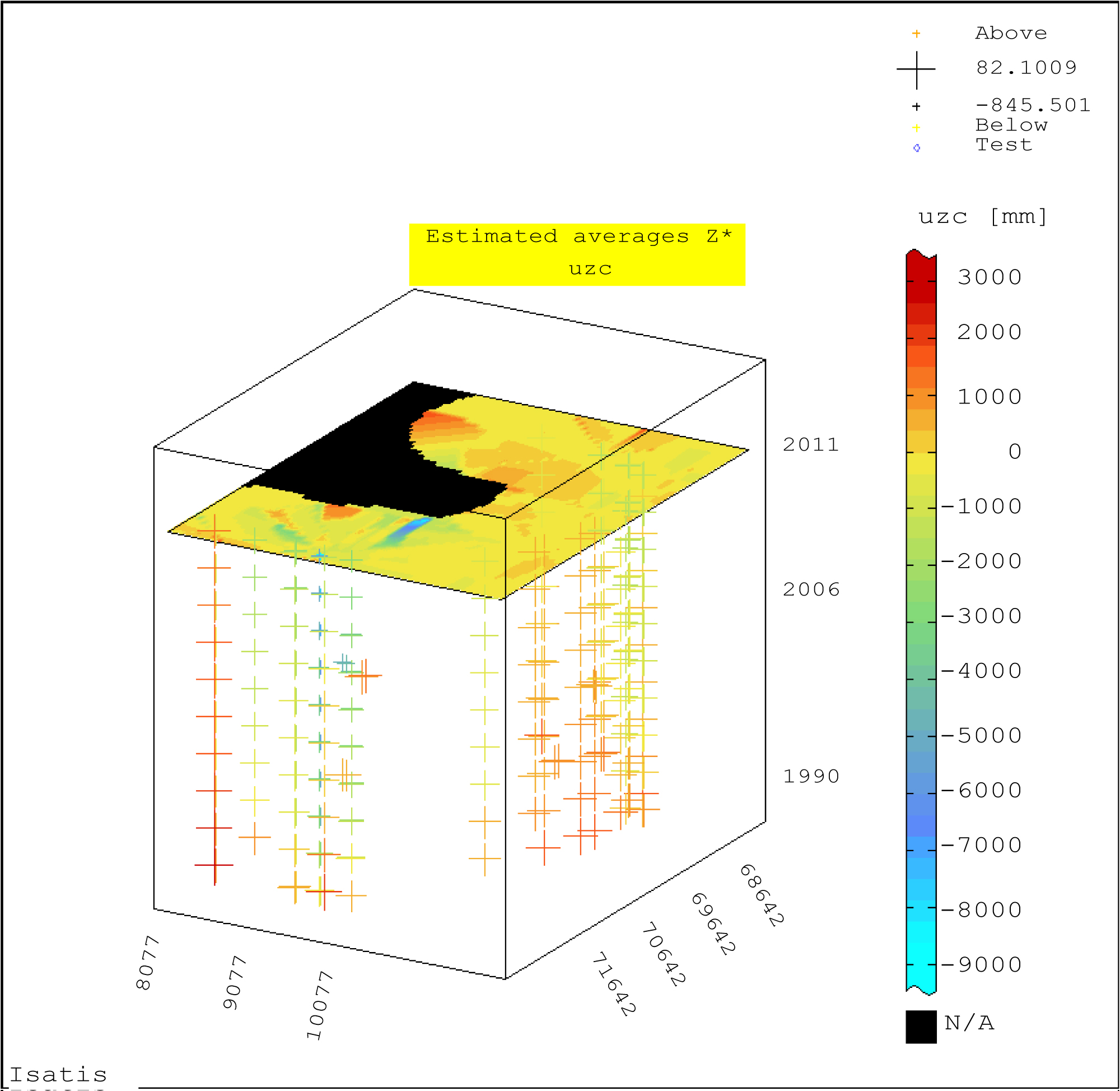
Figure 12: Block-diagram of estimated values Z* of vertical...
Block-diagram of estimated values Z* of vertical displacements uzc of BMs in the hydrotechnical facility (year 2011); ordinary (block) kriging; moving kriging neighborhood.
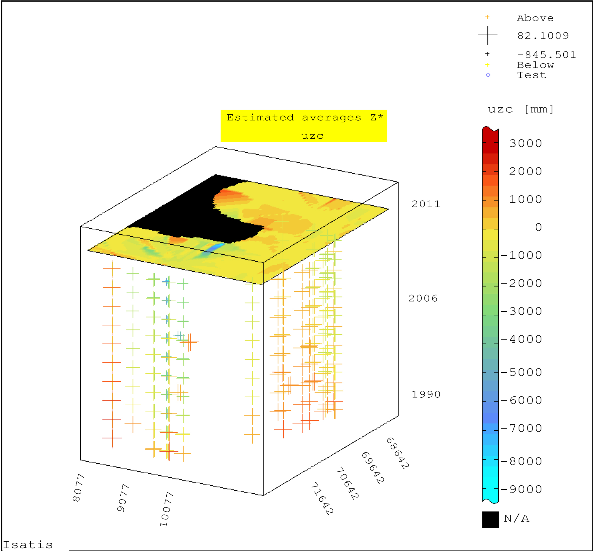
Figure 13: Block-diagram of forecasted values Z* of vertical....
Block-diagram of forecasted values Z* of vertical displacements uzc of BMs in the hydrotechnical facility (year: 2012); ordinary (block) kriging; moving kriging neighborhood.
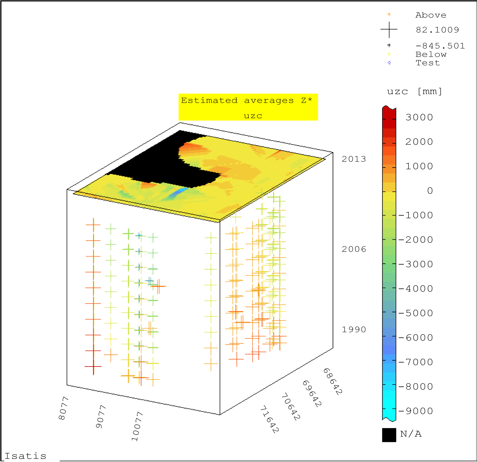
Figure 14: Block-diagram of forecasted values Z* of...
Block-diagram of forecasted values Z* of vertical displacements uzc of the BMs in the hydrotechnical facility (year: 2013); ordinary (block) kriging; moving kriging neighborhood.
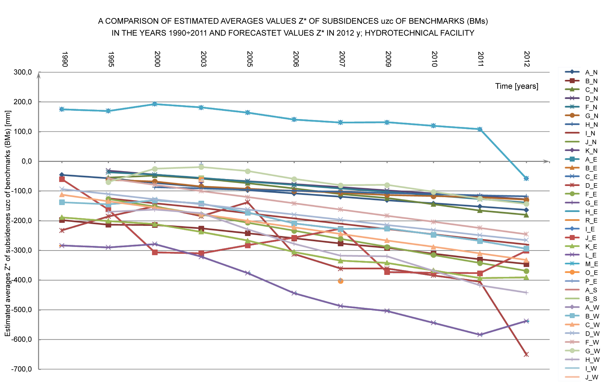
Figure 15: A comparison of estimated averages values....
A comparison of estimated averages values Z* of subsidences uzc of the BMs on the dams (N, E, S, W) of hydrotechnical facility in the years 1990 ÷ 2011 and forecasted values for 2012 y.
Tables
Table 1: Basic statistics of monitored total vertical displacements (uzc) of the BMs in the hydrotechnical facility (years: 1990 ÷ 2011).
Table 2: Basic statistics of monitored displacements Z of the hydrotechnical facility (time database, years: 1990 ÷ 2011).
Table 3: Geostatistical parameters of theoretical models of directional semivariogram of vertical displacements uzc of the BMs (along the time axis: years: 1990 ÷ 2011); hydrotechnical facility.
Table 4: The results of cross-validation of the assumed theoretical model of directional semivariogram of vertical displacements uzc (years: 1990 ÷ 2011) of BMs; assessment errors in the BMs); hydrotechnical facility.
Table 5: A comparison of statistics of estimated averages Z* of vertical displacements (subsidences) uzc of the BMs (years: 1990, 2011) with the forecasted values Z* (years: 2012, 2013); hydrotechnical facility.
Table 6: A comparison of original statistics of vertical displacements (subsidences) uzc of deep repers with estimated values Z* estimated in the nodes of spatial elementary grid (3D); temporal database (years: 1990 ÷ 2011); hydrotechnical facility.
Table 7: A comparison of estimated averages values Z* of subsidences of benchmarks against measured values Z of displacements and values of estimation errors; hydrotechnical object, 2007 y; the assumed theoretical model of directional semivariogram of displacements; ordinary (punctual) kriging, the moving kriging neighborhood.
Table 8: A comparison of estimated averages values Z* of subsidences of BMs points against measured values Z of displacements and values of estimation errors; hydrotechnical object, 2011 y; the assumed theoretical model of directional semivariogram of displacements; ordinary (punctual) kriging, the moving kriging neighborhood.
Table 9: Forecasted values Z* of subsidences of the BMs with temporal overtaking for 2012 y, against original values Z (2011) and estimated values Z* (2011) in measured points of hydrotechnical facility (model of directional semivariogram of displacements; ordinary (punctual) kriging; moving kriging neighborhood.
Table 10: Forecasted values Z* of subsidences of deep benchmarks, with temporal overtaking for 2007 y, against estimated averages values Z* (2006) and original values Z coming from geodetic monitoring (2006, 2007 years) in the measured points (BMs) located in the subsoil of hydrotechnical facility (model of directional semivariogram of displacements; ordinary (punctual) kriging; moving kriging neighborhood.
References
- Namysłowska-Wilczyńska B, Wynalek (2011) The analysis of vertical displacements for a hydrotechnical facility using geostatistics. Pt. 1, Structural analysis and estimation of displacements. Studia Geotechnica et Mechanica 33: 33-54.
- Namysłowska-Wilczyńska B, Wynalek J (2011) The analysis of vertical displacements for a hydrotechnical facility using geostatistics. Pt. 2, Determining the probability of displacement occurrence and its prediction. Studia Geotechnica et Mechanica 33: 67-75.
- Namysłowska-Wilczyńska B, Wynalek J (2014) Spatial analysis of the displacement field based on geodetic monitoring. In: Infobase: Inspiration - Integration - Implementation: VII National Scientific Conference, Gdańsk - Sopot, 8-10 September 2014. Gdansk University of Science and Technology, Gdansk, 1-12.
- Namysłowska-Wilczyńska B, Wynalek J (2017) Geostatistical investigations of displacements on the basis of data from the geodetic monitoring of a hydrotechnical object. Studia Geotechnica et Mechanica 39: 59-75.
- Namysłowska-Wilczyńska B, Wynalek J (2018) Prediction of short-term displacements of hydro-engineering structure. In: XXVII Scientific and Technical Conference: Geodesy, construction, environment-scientific, legal, practical and didactic aspects. Book of Abstracts, Rzeszow, Rzeszow University of Science and Technology., Faculty of Civil and Environmental Engineering and Architecture, 25.
- Bielecka E (2006) Geographic information systems - theory and applications. PJWSTK Publisher, Warsaw.
- Myrda G, Litwin L (2005) Geographic information systems. Spatial data management in GIS, SIP, SIT, LIS. Publisher Helion, Gliwice.
- Osada E (1998) Geo-data analysis, alignment and modeling. Agricultural University, Wroclaw.
- Pilz, Jurgen (2009) Interfacing Geostatistics and GIS. Springer Berlin Heidelberg, Berlin, Heidelberg.
- Szczepanek R (2017) Spatial information systems together with QGIS. Cracow University of Science and Technology, Publishing House, Cracow.
- Clark I (1979) Practical geostatistics. Appl Sc Publishers, London, 129.
- Journel AG, Huijbregts CJ (1978) Mining Geostatistics. Academic Press, London, New York, San Francisco, USA.
- Kiciak P (2000) Basics of modeling curves and surfaces. Scientific-Technical Publishers, Warsaw.
- Matheron G (1962) Traite de Geostatistique Appliquee: Memoires du Bureau de Recherches Geologique et Minieres. vd. 14: Editions Technip. Paris, 333.
- Mucha J (1994) Geostatistical methods in documenting deposits. Cracow University of Science and Technology, Publishing House, Cracow, 155.
- Namysłowska-Wilczyńska B (1993) Variability of copper ore deposits in the Foresudetic Monockline against the background of geostatistical methods. Scientific Works, Institute of Geotechnics and Hydrotechnics, Wroclaw University of Science and Technology No. 64, Monographs no 21, Wroclaw, 207.
- Namysłowska-Wilczyńska B (2006) Geostatistics theory and applications. Publishing House of the Wrocław University of Science and Technology, Wroclaw, 365.
- Namysłowska-Wilczyńska B (2008) Modeling of Hydrological Processes. Collective work Publishing House, Wroclaw University of Science and Technology, Wroclaw, 526 Modeling and forecasting (3D) of precipitation and SO4-sulfate content in precipitation in the central Odra river basin using geostatistics, 35-74.
- Suchecka J (2014) Spatial statistics. Methods for the analysis of spatial structures. CH Beck, Scientific Editors, 222.
- Wackernagel H (1995) Multivariate geostatistics. Springer-Verlag Berlin, Heidelberg, New York, 256.
- Namysłowska-Wilczyńska B, Skorupska B, Wieniewski A (2012) Geostatistical analysis of the variability of technological parameters of ash slag deposited at the industrial waste landfill. Environmental Protection 34: 43-48.
- Namysłowska-Wilczyńska B (2012) Geostatistical methods used to estimate Sieroszowice copper ore deposit parameter. Journal for the Geological Sciences 40: 329-361.
- Namysłowska-Wilczyńska B (2013) Geostatistical hydrogeochemical 3D model for Kłodzko underground water intake area. Part I. Estimation of basic statistics on quality parameters of underground waters. Studia Geotechnica et Mechanica 35: 157-182.
- Namysłowska-Wilczyńska B (2016) Space-Temporal Variation in Underground Water Some Quality Parameters in Klodzko Water Intake Area Using Statistical and Geostatistical Methods (SW Part of Poland). Journal of Geological Resource and Engineering 3: 105-124.
- Namysłowska-Wilczyńska B (2016) Geostatistical analysis of space variation in underground water various quality parameters in Klodzko water intake area (SW part of Poland). Studia Geotechnica et Mechanica 38: 15-34.
- Namysłowska-Wilczyńska B (2018) Filtration of components of sieroszowice mine copper ore deposit variogram models by means of estimation ordinary kriging technique. Geoinformatics & Geostatistics: An Overview 6.
- Namysłowska-Wilczyńska B (2019) Application of some kriging techniques aimed at the integration of environmental parameters for the improvement of estimation quality. Proceedings of the 7th International Symposium on Geotechnical Safety and Risk (ISGSR), Taipei, Taiwan, 11-13. 309-314.In: Jianye Ching, Dian-Qing Li and Jie Zhang, Research Publishing, Singapore.
- Namysłowska-Wilczyńska B (2019) Application of geostatistical techniques for the determining of an anomalous zones of copper ore deposit in the area of Polkowice mine. Geoinformatics & Geostatistics: An Overview 7.
- Bogusz J, Kłos A, Grzempowski P, Kontny B (2014) Modelling the velocity field in a regular grid in the area of Poland on the basis of the velocities of European permanent stations. Pure and Applied Geophysics 171: 809-833.
- Chien-Kuan Li, Kuo En Ching, Chen Kwo-Hwa (2019) The ongoing modernization of the Taiwan semi-dynamic datum based on the surface horizontal deformation model using GNSS data from 2000 to 2016. Journal of Geodesy 93: 1-16.
- Ghiasi Y, Nafisi V (2015) The improvement of strain estimation using universal kriging. Acta Geodaetica et Geophysica 50: 479-490.
- Hang ZJ, Yao N (2008) The Geostatistic Framework for Spatial Prediction. Geo-spatial Information Science 11: 180-185.
- Ligas M, Szombara S (2018) Geostatistical prediction of a local geometric geoid - kriging and cokriging with the use of EGM2008 geopotential model. Studia Geophysica et Geodaetica 62: 187-205.
- Valizadeh Nariman, Mirzaei Majid, Allawi Mohammed, Afan Haitham, Mohd Nuruol, et al. (2017) Artificial intelligence and geo-statistical models for stream-flow forecasting in ungauged stations: State of the art. Natural Hazards 86: 1377-1392.
- Ma YZ (2019) Quantitative geosciences: Data analytics, geostatistics, reservoir characterization and modeling. Cham: Springer International Publishing.
Author Details
Barbara Namysłowska-Wilczyńska* and Janusz Wynalek
Wroclaw University of Science & Technology, Wrocław, Poland
Corresponding author
Barbara Namysłowska-Wilczyńska, Wroclaw University of Science & Technology, Wybrzeże Stanisława Wyspiańskiego 27, 50-370, Wrocław, Poland.
Accepted: April 23, 2020 | Published Online: April 25, 2020
Citation: Namysłowska-Wilczyńska B, Wynalek J (2020) Spatial-Temporal Analysis and Short-Term Forecasting of Hydrotechnical Facility Displacements. Int J Earth Sci Geophys 6:033
Copyright: © 2020 Namysłowska-Wilczyńska B, et al. This is an open-access article distributed under the terms of the Creative Commons Attribution License, which permits unrestricted use, distribution, and reproduction in any medium, provided the original author and source are credited.
Abstract
Methods of applied (spatial) statistics enable the analysis of measurement data. This paper presents research methods aimed at applying geostatistics, i.e., anisotropic (directional) variogram, ordinary (block) kriging and point ordinary (point) kriging to the spatial analysis of geodetic data. An investigative approach, which can be used for the space-time analysis of the displacements (and even deformations) of any small- and large-area facility being under geodetic monitoring, is proposed.
Changes in the displacements of check points on a hydrotechnical facility are analysed in both the area and time domain in order to assess the structure's behaviour and safety condition throughout its entire service life.
It is recommended to determine how the values of the investigated displacement (Z) parameters are distributed also in unsampled places and demarcate the critical subareas characterized by great variation in displacement values, indicative of possible local deformations.
The subject of spatial analysis was the time database of displacements for the analyzed hydrotechnical object, developed for the years 1990÷2011. This database contains original displacement values, controlled points. As part of this study, displacements are forecasted for a small set of check points (n = 29) in selected locations on a large hydrotechnical facility while interactively performing kriging calculations, taking into account monitoring data (n = 268) for the period 1990÷2011. Forecasted values Z* and forecast standard deviation σk were calculated two years in advance for the next measurement epoch, using the directional variogram function and ordinary point kriging.
The area-time forecast made it possible to determine the forecasted short-term displacements Z*, taking into account the history and dynamics of the displacement process, i.e. displacements Z recorded in the previous years. In this way values Z* in the particular periods of the service life of the structure can be estimated when there occurs high variation in displacements Z.
Keywords
Hydrotechnical facility, Subsoil, Geodetic monitoring, Vertical displacements (subsidences, settlements), Benchmarks BMs (repers), Variation, Estimating, Forecasting, Space-time forecast, Anisotropic semivariogram, Ordinary (block, point) kriging
Introduction
Displacements in broadly understood research problems encountered in geodetic analyses are usually forecasted analytically by calculating, i.e., the rates at which the check points on water control structures displace, using data from geodetic monitoring conducted in consecutive measurement epochs [1-5]. GIS applications can generate maps of the probability of the occurrence of deformations, especially for macroareas located within the range of mining impacts [6-10]. Geostatistical techniques have been used so far to forecast displacements in space-time, to a smaller extent. Therefore the authors devote this paper to this problem.
By applying geostatistical methods one can accurately model spatial data, estimations and estimation accuracy and so determine the reliability of the estimation results [8,11-20]. For years geostatistical methods have been used in geological sciences, mining, environmental protection, agriculture, geochemistry, epidemiology, meteorology, oceanography, forestry and materials science, to a lesser or greater extent [15-18,21-28] and also in geodesy [29-34]. They are also used in thematic cartography, e.g. to mapping hydrocarbon reservoirs, and in the oil and natural gas extraction industry [35]. In hydrogeology, they are used to model the properties (permeability and porosity), geometry and hydraulic parameters of aquifers and to assess the pollution of the soil-water environment, soils and groundwater, f.g. by heavy metals content [18,23-25].
The aim of this research was to produce a short-term space-time forecast of the displacements of a large hydrotechnical object [4,5]. Because of their spatial character (stemming from the distribution of check points on the structure) and their time character (deriving from geodetic monitoring conducted over years), the considered displacements were subjected to space-time analyses. An important aspect of this research was to carry out a space-time analysis of the displacements not only in order to assess and interpret them in a selected measurement epoch, but also to explore the possibility of making a short-term (one year) forecast of the structure's displacements before the scheduled geodetic monitoring.
The results of the geostatistical spatial analyses of measuring data reflecting the monitoring of vertical displacements of a small hydrotechnical facility - weir Opatowice on Oder river, in Wroclaw (Poland), were presented in two articles published, in Part I and Part II, in 2011 [1,2].
Isotropic and directional variograms, the ordinary block kriging method and the techniques of quick interpolation, i.e. the inverse distance squared method and the linear kriging model were used. In further analyses, indicator geostatistics, i.e. indicator variograms and indicator probability maps for particular thresholds were applied [1,2]. This allowed determining the subregions with various susceptibilities to exceeding particular probability thresholds of local deformations occurrence. The effect of geostatistical studies was the cartographic characteristic of the displacements in the Opatowice weir [1,2]. Probabilities maps enabled to predict the significant risk areas associated with a possible change in the geometry of the hydrotechnical object, i.e., its local deformation. A spatial-time prognosis in successive periods of the facility operation, was also made. The forecasted values Z* of displacements for the following year (1999), with reference to the history of this process, i.e. the estimation from prior years (1987, 1991), were determined [2].
Using selected geostatistical methods, Authors have dealt with interesting and current issues connected to space-time analysis, modeling displacements and deformations, as applied to large-area hydrotechnical object, on which geodetic monitoring, at a macro-regional scale, is conducted, situated in SW part of Poland, and obtained results were in earlier work published in 2017 [4].
Using ordinary (block) kriging the values of the Z* estimated averages of displacements were calculated together with the accompanying assessment of uncertainty - a st. deviation of estimation σk. Raster maps of the distribution of averages Z* and st. deviations σk were obtained for years 1995 and 2007, taking the ground height 136 m a.s.l. into calculation. Methods of quick interpolation were also used, such as the inverse distance squares, a linear model of kriging, a spline kriging, which made the recognition of the general background of displacements possible (without the accuracy assessment of Z* value estimation, of σk, related to 1995 and 2007 and the elevation. As a result of applying these techniques, clear boundaries of subsiding areas, upthrusting and also horizontal displacements on the examined hydrotechnical object were marked out, which can be interpreted as areas of local deformations of the object, important for the safety of the construction [4].
In the present article, estimating and forecasting of vertical displacements (subsidences) were carried out for a large hydrotechnical facility, situated in SW part of Poland, one from the biggest object in Europe, taking into account an irregular network of measurement points carried out in the years 1990 ÷2011, in 35 locations [5].
All calculations connected with spatial analyses were performed using geo-statistical packet of software ISATIS, Geovariances Firm, Avon-Cedex, Fontainebleau, France.
Object and Subject of Research
The hydro-engineering structure (a sump reservoir of flotation tailings) is located in the SW part of Poland, between Lubin and Głogów, at the distance of 80 km from Wroclaw in the Lower Silesian Province (Figure 1). It is situated in a natural valley in a morphological depression between moraine hills of Pleistocene glaciations in the SE part of Dałków hills (which regionally constitute a part of the Silesian Wall), in the upper part of the Rudna River catchment area, in the Kalinówka Stream valley. Initially the sump reservoir was bounded with an east (E) dam and a west (W) dam, closing the natural valley. Since the north dam (N) and the south (S) dam were built the total length of the dams bounding the reservoir amounts to about 14.4 km. In the middle part of the reservoir there is a supernatant water pond 624 ha in area (and beaches (770 ha)), collecting water draining from the silting up flotation tailings. The depth of water (above the sediment level) in the pond is 2.5 m. The total volume of the reservoir amounts to 700 mm3, including the water collected in the pond (8 mm3). Currently, the reservoir is at the stage of formation up to the elevation of 185 above sea level. The dams (embankments) are 20-60 m high. The reservoir waste storage capacity is 657 mln. m3 (the annual buildup amounts to about 26 mm3). Operational estimates indicate that the reservoir would fill up in 2023. The facility is being enlarged not only upwards (by increasing the height of the dams), but it also became necessary to add a south (S) sector (under construction). It is estimated that after the existing facility is extended upwards to 195 m a. s. l. and sector S is enlarged to 600 ha (by 2021), to ultimately hold 170 mm3 of tailings, it will be possible to develop the reservoir's capacity to 1.1 milliard m3 and operate it safely by as late as 2042. Currently the whole facility occupies the area of nearly 14.1 km2 and it is the largest facility of this kind in Europe and one of the largest in the world. The location and a general view of the facility is shown in Figure 1.
The subject of the spatial analyses, carried out here using some geostatistical methods, were vertical displacements uzc of the subsoil under the crest of the dams of the analysed hydro-engineering structure.
The deep-seated benchmarks (BMs) (control points) are surveying elevation markers monumented in the native subsoil under the crest of the hydro-engineering structure, on the W, N, E and S dams (without the foreland).
In the geostatistical studies of the changes in displacements over the years 1990-2011 the total number of monitored deep-seated benchmarks on the structure ranged from 16 points (1990) through 26 (1995) and 29 (2007) to 35 (2003), while in the years: 2000, 2005, 2006 and 2009-2011 it remained at the level of 27 points.
A base map (Figure 2a) and a block diagram in - perspective (Figure 2b) showing the distribution of the deep-seated BMs in the subsoil of the structure's crest and their vertical displacement over the ten-year period of geodetic monitoring are presented (1990, 1995, 2000, 2003, 2005, 2006, 2007, 2009, 2010, 2011).
Research Methods
The basis for the spatial analyses was a temporal 3D database containing the vertical displacements of the monumented BMs in maximally 35 locations in the subsoil of the reservoir's crest for the years 1990 ÷ 2011 (n = 268).
Analysing the variation in the displacements, first the basic statistics (the minimum Xmin and maximum Xmax values, the arithmetic mean , the standard deviation S and the coefficient of variation) V were evaluated. In addition, a displacement distribution histogram, skewness coefficient g1, kurtosis coefficient g2, quantiles Q1-25, Q2-50, Q-75 and a boxplot were calculated.
Then, a directional (anisotropic) variogram along the time axis (1990 ÷ 2011) was determined and its pattern was modelled using theoretical functions. The model parameters were the basis for estimations conducted using the ordinary (block) kriging technique. For this purpose the considered area was covered with a grid of elementary blocks (sect. 7). Estimated averages Z* and estimation standard deviation σk were determined for the centres of the grid blocks.
Finally, using ordinary point kriging, displacement values Z* in the selected points of the considered area were estimated and forecasted for the selected years (2007, 2012) and the value of σk was calculated. The calculations were based on the parameters of the variogram model along the time axis.
The relevant formulas relating to the methods and techniques used in this paper can be found in different publications, e.g., in [4,11,12,14-17,19,20,26].
Evaluation of Basic Statistics of Displacements
The original data on the monitored vertical displacements of the deep-seated benchmarks (BMs) on the hydro-engineering structure in the years 1990 ÷ 2011, contained in the temporal (3D) geodetic database, were subjected to a preliminary statistical assessment. Altogether 268 measurement data for the analysed years were subjected to the displacement variation analysis.
The results of the assessment of the basic statistics concerning total vertical displacements uzc of the control points on the hydro-engineering structure for the particular years of geodetic monitoring are reported in Table 1, while the results for all the measurement data contained in the temporal database are presented in Table 2.
These were original vertical displacement data Z (uzc) from ten year long geodetic monitoring (1990, 1995, 2000, 2003, 2005, 2006, 2007, 2009, 2010, 2011) of the BMs (Table 1).
It is apparent that in the years 1990-2011 subsidence values consistently increase from -234.0 mm in 1990, through -589.6 mm in 2003 (at the maximum number (35) of deep-seated BMs on the structure) to -845.5 mm in 2011 (the largest subsidence in the geodetic monitoring history). A similar tendency as in the case of total vertical displacements uzc of the BMs on the structure, is also observed for average values, which changed from -98.0 to -275.9 mm over the years 1990 ÷ 2011.
The coefficient of variation (V) of the original total displacements of the deep-seated benchmarks remained at the level of about 55 - 70% over the analysed years. The considerably high values of V indicate high displacement variation due to the changing operating conditions in the facility, but also to the varied geotechnical conditions in the subsoil in which the deep-seated benchmarks were monumented. Considerably higher values of variation coefficient V were obtained for the earlier years, i.e. 1990 and 1995, whereas the ones for the later years (beginning from 2005) were lower.
The basic statistical parameters of the displacements for whole time monitoring period (together) (1990 ÷ 2011) were inserted in Table 2.
The coefficient of variation (V) ~-69% based on the geodetic monitoring data, indicates substantial changes in the displacements of the BMs in the considered period of 1990÷2011 (Table 2), similarly for years 1990, 1995 and 2000 (Table 1).
Figure 3 shows the variation in the displacements (settlements) uzc of the particular MBs located on the (N, E, S, W) dams of the hydrotechnical object, based on the original geodetic monitoring data for the years 1990÷2011.
A single graph in the diagram shows changes in the displacement of a particular permanent bench mark on a given dam over the years. One can see that on the whole facility the settlements of the particular BMs steadily increase up to 2011, which can also be seen in Figure 4 showing the monitored displacements of the PMBs on only dam E.
An empirical histogram of the distribution of vertical displacements uzc of the deep-seated benchmarks is shown in Figure 5a, Figure 5b and Figure 5c. The histogram is characterized by moderate negative asymmetry, and negative skewness coefficient g1 amounts to -1.52. The histogram exhibits a leptokurtic character and kurtosis coefficient g2 reaches the value of 6.53 (Figure 5a). The negative skewness stems from the character of the analysed vertical displacements (uzc) of the control points on the structure over the considered temporal perspective. Most of the original values of total vertical displacements uzc have the character of subsidences. It was only in the initial period of the control surveys that small ground heaves, amounting to +82.1 mm (1990) and +41.1 mm (1995), which subsided and turned into subsidences of the control points on the structure in the subsequent years, were observed (Table 1).
In the boxplot one can see outlier values, shown against the displacements and the arithmetic mean positions, reflecting the wide range of subsidence values in the analysed period of time (Figure 5b).
Q-Q Plot Quantile indicates on relatively a good fitting the experimental distribution of displacements with the Gaussian distribution (Figure 5c).
Variogram Modelling
In the next step of the analysis a directional anisotropic variogram calculated along the analysed time interval (the years 1990÷2011), i.e. direction normal to the reference plane and its course was approximated with the sum of theoretical models (Figure 6).
In the calculations of this variogram, 268 point data were taken from the time base (3D) of vertical displacements, measured maximally in 35 locations.
This variogram shows the directional non-stationary changes in the considered parameter - the vertical displacements (uzc) of the BMs on the structure (Figure 6). Generally, over the analysed years (1990÷2011) the displacement parameter shows a marked growing tendency. In the initial part of the diagram (years 1990÷2005) function γ(h) reaches the lowest (almost identical) values and then (years 2005÷2011) the function values sharply increase. The sharpest increase in the values of function γ(h) takes place in the end part of the diagram, last green point, which was calculated on the basis of a very small number of sample pairs (n = 15), therefore it can be omitted in the interpretation.
The observed variogram pattern stems from the behaviour, variation of displacement (subsidences) values, i.e. Xmin, Xmax, mean , over the analysed period of 1990 ÷ 2011, which consistently increase beginning from 2003 (Table 1).
The course of the empirical directional variogram was approximated with a complex (theoretical) geostatistical model consisting of three theoretical functions, i.e. two spherical models and a power model (by means of automating fitting) (Table 3 and Figure 6). Small random factor (nugget effect C0) is involved in the general variation C of the investigated displacement parameter. Influence ranges a, determined on the basis of the adopted spherical models, are: a = 1 year and a = 1 year, which indicates that the displacement values are mutually correlated within such time intervals. For power model the scale parameter amounting 9 was obtained.
Results of Cross-Validation of Theoretical Variogram Model
Next cross-validation calculations were carried out to verify the adopted theoretical directional variogram model consisting of spherical, spherical and power structures for vertical displacements (Figure 7a, Figure 7b, Figure 7c and Figure 7d).
A very high coefficient of correlation between the original values Z and the estimated values Z* of PBM displacements, amounting to r = 0.97 (and so close to 1) (Figure 7a), was obtained.
The base map shows that in some locations there is a small number of points whose displacement values differ from those of the other displacements in the set (Figure 7b).
The histogram of standardized estimation error probability density shows a slight left-side asymmetry (negative skewness), which indicates a very small underestimation of this error (Figure 7c).
In the diagram of estimated averages Z* and standardized estimation error values one can see only few divergent estimated averages Z*. The largest standard errors correspond to the divergent (being outside the assumed confidence level) values of estimated averages Z* in the range of -400 mm÷-300 mm (settlements of BMs), (Figure 7d).
When the total number of (testing) data (n = 267) was taken into account in the calculations, the standardized error variance amounted to 1. When the number of data was a little smaller (n = 262), i.e. after the divergent values had been rejected, the error variance decreased to 0.524 (Table 4).
Summing up, the cross-validation results indicate a very good fit of the theoretical model to the course of the empirical semivariogram. Variance of standardized error amounts to 1, i.e., the reference value (Table 4).
Results of Estimation Using Ordinary (Block) Kriging
A space-time forecast was made on the basis of a small set of check points, in the form of benchmarks (PBMs), monitored on the water control structure, taking into account the full time series of data (n = 268) for the years 1990÷2011. The data contained in the time database, i.e. total vertical displacements uzc of the PBMs, whose number increased in the successive years of water control structure service life, amounting to from several to a few tens points (maximally 35 benchmarks), were used in the calculations.
The 3D elementary grid adopted for estimating and forecasting the vertical displacements of the deep-seated BMs on the hydro-engineering structure, using block and point kriging and taking the data time series (n = 268) into account, was superimposed on the analysed area (Figure 8a). Figure 8b, Figure 8c and Figure 8d show planes XOY, XOZ and YOZ for the analysed structure. There were 3850 elementary blocks on a plane and 46200 (77 × 50 × 12) blocks in the 3D systems. The dimensions of a single grid cell (mesh) were 50 × 100 × 1 year.
When estimating and forecasting values Z* of total displacements uzc, using ordinary (block) kriging, a moving kriging neighbourhood (a subarea of the search for samples: minimum number of samples - 4; number of horizontal angular sectors - 8; optimum number of samples - 3) was assumed. This means that 24 samples coming from the subarea were taken into account when estimating a given grid node.
The averages Z* of BMs' displacements for the particular years of geodetic monitoring (1990÷2011), taking into account the theoretical directional semivariogram model values (D-90 - along the time axis), were estimated in 3165 nodes of a spatial elementary grid covering the considered area of the water control structure.
Table 5 presents estimated averages Z* displacements, using the ordinary (block) kriging method, for selected years of monitoring, i.e. 1990, 2011, and also for the years 2012 and 2013 of forecast (prognosis) performing.
The arithmetic mean values Z* determined on the basis of the estimated averages Z* displacements differ significantly for the years 1990 and 2011 (Table 5). The same statement relates to Xmin and Xmax values. Meantime mean from averages Z*, calculated for 1990 is much smaller, in relation to subsequent years, when subsidences increase (Table 5).
The mean values determined on the basis of the forecasted averages Z * are higher for the years 2012÷2013 (especially for 2013), in comparison to 2011 (Table 5).
As in the case of other statistics, the coefficients of variation V reach very large values and are similar for the years 2011÷2013 (Table 5). A very high coefficient of variation V was obtained for 1990, which may result from the much smaller size of original data Z that was available in comparison to other years. Generally, large values of V coefficients reflect a large variability of the estimated values Z* of displacements, calculated in 3165 nodes of the assumed spatial elementary grid.
A comparison of the original data (Z) on vertical displacements uzc, measured in 268 points over 10 years (Table 2), for the particular years of geodetic monitoring (1990÷2011), with the averages Z* calculated in 3165 nodes of the whole elementary grid (3D) shows large changes in the settlements, in particular years, as indicated by the very high respective variation coefficients V (Table 5), if we are using block ordinary kriging for estimating.
The estimated averages Z*, calculated on the basis of theoretical model parameters (semivariogram D-90, years 1990÷2011), using the ordinary block kriging method, were smoothed from theoretical reasons (connected with used kriging technique) and so they cannot be directly related to the statistics calculated on basis of the original Z data.
The averages Z* of PBM displacements for the particular years of geodetic monitoring (1990÷2011), taking into account the theoretical directional semivariogram model values, were estimated in 35280 nodes of a spatial elementary grid (3D) covering the considered area of the water control structure. The statistics on displacements Z*, estimated using ordinary block kriging, are presented against the background of the original monitored displacements Z in 268 PMB locations over the years 1990-2011 in (Table 6).
A comparison of the original data (Z) on vertical PBM displacements uzc, measured in 268 points over 10 years, with the averages Z* calculated in 35280 nodes of the spatial elementary grid shows very large - minimal values - Xmin and Xmax of estimated values Z* of settlements, as indicated by the respective variation coefficients V. The value of V is higher in the case of the estimated values Z* is connected with a very big count (size) N of assumed elementary grid nodes, i.e. N = 35280 (Table 6).
The estimated averages Z*, calculated for 35280 grid nodes using the ordinary block kriging method, were smoothed for theoretical reasons (resulting from the used kriging technique) and so they cannot be directly related to the statistics calculated on basis of the original Z data.
However, a lower value of mean , based on the estimated values Z*, for one of grid nodes, compared to the mean of original values Z, was obtained (Table 6).
Owing to the fact that ordinary block kriging was used to estimate settlements, raster maps of the displacements of the BMs, calculated for the consecutive years of the analysed water control structure could be plotted.
The estimated values Z* of the vertical displacements uzc of the BMs on the water control structure in 1990, 2005, 2006, 2011 are shown graphically in Figure 9, Figure 10, Figure 11 and Figure 12.
Then average Z* settlements were forecasted by means of ordinary block kriging for years 2012 and 2013. The data from the geodetic monitoring of the displacements for the years 1990÷2011 were used in the calculations. The calculation results are presented in Figure 13 and Figure 14.
A block-diagram drawn up for 1990, within the analyzed object, can be seen both sub-areas of smaller and large displacements, which are sub-areas of elevations and the largest subsidences. These sub-areas are found within the Eastern Dam of the hydrotechnical facility. In the rest of the object, the variability of displacement values is smaller (Figure 9).
On the block diagram calculated for 2011, the image of the estimated Z* displacements changes radically. New subareas appear with larger displacements of larger sizes, some overlap with those separated for 1990, while zones with larger subsidences change their location (Figure 9 and Figure 12).
The block diagram obtained for the Z* forecasted values in 2012 confirms the previously observed tendency of changes in 2011. The subsidence and elevation zones occur in almost identical locations (Figure 13).
The block of forecasted values Z* for 2013 shows a similar tendency of changes, with the difference that new details of variability can be found, related to the appearance of new small zones of larger (or smaller?) settlements ? (subsidences), however these differences are subtle (Figure 14).
Generally, the behaviour of the estimated averages Z* of the BMs' settlements (Figure 15) is a reflection of the tendencies in the changes of the monitored values Z (Figure 3). The settlements slowly increase over the years. The divergences observed for some points (where settlements increase or decrease) can be ascribed to the nature of the variation of the measured displacements and to the peculiarity of the kriging method (the smoothing effect). It should be noted that in 2011 the trend for estimated settlement averages Z* (in the grid nodes) was similar to that for monitored values Z (in the measuring points), (Figure 3).
It appears that in 2012, as expected (consistently with the trend), lower values of forecasted displacements Z* than those of estimated averages Z* for 2011 were obtained for the particular benchmark locations. The trend indicating intensifying forecasted settlements is visible in Figure 15. Considering the very good cross-validation parameters, the results of the forecast of the benchmark displacements for 2012 seem to be reliable.
Results of Estimating Displacements by Means of Ordinary Point Kriging
The ordinary point kriging technique was applied to the data contained in the time database of the vertical displacements (Z) of the BMs monitored on the water control structure in the years 1990÷2011 to calculate estimated averages Z* of the PBMs displacements in the monitored points for the consecutive years of monitoring and averages Z* forecasted for 2012 and 2013. The estimation and the forecasting were based on the theoretical model of the directional semivariogram of the settlements (along the time axis, 1990÷2011), (Figure 6 and Table 3).
Estimation errors for selected years, i.e. 2007 and 2011, were determined by comparing the estimated averages Z* with the monitored values Z in the particular BMs (differences Z-Z*) and expressed in % and shown in (Table 7 and Table 8).
The largest benchmark settlements (BM-13E: -656.9 mm, BM-2E: -530.4 mm, BM-1E: -500.4 mm, BM-14E: -460.2 mm) were registered on water control structure dam E in 2007. The benchmark settlements on dams N and W are distinctly smaller (Figure 3, Figure 4 and Table 7).
The benchmark settlements Z*, estimated using the ordinary kriging technique and the directional settlement semivariogram model (Table 7), reflect the general tendency in the benchmark settlements monitored on the structure. The highest displacement values Z* show the BMs on the structure's dam E (BM-41E: -486.8 mm, BM-8E: -486.8 mm, BM-1E: -402.6 mm, BM-2E: -399.4 mm), whereas the ones on dams N and W show much lower values.
The average displacement estimation errors, calculated as differences between monitored values Z and estimated values Z*, reach negative and positive values, generally ranging from a few to a few tens mm. Expressed in per cent, they reach values ranging from a few to a few tens %. In some points average estimation errors are large, indicating low and high estimated displacement values Z* relative to monitored values Z.
The largest benchmark settlements were registered on water control structure dam E in 2011 (BM-13E: -845.5 mm, BM-14E: -595.7 mm, BM-41E: -482.9 mm, BM-8E: -397.3 mm), while the ones on dams N and W were distinctly smaller (Figure 3, Figure 4 and Table 8).
The estimated values Z* of the benchmark settlements (Table 8) reflect the general tendency in the settlements of the monitored BMs on the structure. The highest displacement values Z* are shown by the BMs located on the structure's dam E (BM-8E, BM-41E: -583.5 mm, BM-13E, BM-14E: -405.5 mm), whereas the ones obtained for dams N and W are much lower.
The average displacement estimation errors (Z-Z*), having both negative and positive values, generally reach the level of a few mm to a few tens mm. Expressed in percent (%), they reach values ranging from a few % to a few tens %. In some points average estimation errors are large (due to low or high estimated displacement values Z* relative to monitored values Z).
Generally, one can say that the averages Z* of the benchmark settlements, estimated using the ordinary point kriging technique, reflect well the general tendency in the settlements of the BMs monitored on the water control structure in 2007 and 2011 and in the data from the time series for the years 1990÷2011. Comparable results were yielded by ordinary point kriging calculations for the years 1990, 1995, 2000, 2003, 2005, 2006, 2009 and 2010.
Space-Time Forecast of Displacements, Made Using Ordinary Point Kriging
Subsequently, an attempt was made to forecast the settlements a year in advance, i.e. for 2012 and 2013, on the basis of the data from the time series for the years of monitoring 1990÷2011.
The forecasted values Z* of the benchmark settlements for 2012 were compared with the estimated values Z* for 2011 and the forecasted displacement increments were estimated on the basis of the Z*2012 - Z*2011 differences and then expressed in % (Table 9).
By comparing the forecasted benchmark settlements Z* for 2012 with the estimated values Z* for 2011 it was only possible to estimate (with regard to the value and the sign) the relative forecasted increments (Z*2012 - Z*2011) in the settlements of the BMs for 2012. Due to monitoring inaccuracy, the positive and negative relative increments in the forecasted displacements (uplifts and settlements of the BMs), up to 10÷20 mm in size, reflect insignificant changes in the position of the BMs on the structure, while the larger relative increments (above a few tens mm in size) may indicate a significant character of the forecasted displacements of the BMs on the structure (Table 9).
In order to verify the forecasted relative increments in the displacements of the BMs for 2012 it would be interesting to compare the original displacement values Z registered in 2011 with the original data Z from monitoring in 2012, by determining the absolute increments in benchmark displacements on the basis of the Z2012 - Z2011 differences. However, at the moment the authors do not have the relevant data.
For this reasons the authors made an attempt to verify the forecasted benchmark displacements on the basis of the available geodetic monitoring data from previous years, using a reduced time database and the original data from a shorter time series for the years 1990÷2006.
Similarly as above, a forecast of BMs' displacements was made one year in advance, but this time the values of the forecasted displacements were determined for the year 2007 for which displacement values from geodetic monitoring were available.
Table 10 shows the forecasted relative increments in benchmark displacements, estimated on the basis of the differences between the forecasted settlements Z* for 2007 and the estimated settlements Z* for 2006 (Z*2007 - Z*2006), and the absolute increments in displacements, calculated as part of the verification process on the basis of the differences between the available original values of the benchmark displacements for 2007 and the monitored values of benchmark settlements for 2006 (Z2007 - Z2006). In addition, forecast errors in the measuring points (Z2007 - Z*2007) were calculated.
It appears from the verification of the forecast benchmark displacements that the results of the forecast made one year in advance for 2007 describe well the character, and even the scale, of the actual changes in the position of the check points on the structure, showing their tendency towards settlement. This is confirmed by both the original benchmark settlements registered by geodetic monitoring in the whole time series of 1990÷2006 and the ones registered in 2007 (Figure 3, Figure 4 and Table 10).
The forecasted increments in benchmark displacements, calculated on the basis of the estimated differences Z*2007 - Z*2006, are slightly overestimated in comparison with the absolute displacement increments (Z2007 - Z2006) determined through verification (on the basis of the original values known from geodetic monitoring conducted in 2007 and 2006). Such calculation results represent well the phenomenon of the forecasted settlements of the check points on the water control structure.
The values of the settlements forecasted for 2007 (Z*2007) are not significantly different from the ones monitored in 2007 (Z2007). An analysis of the forecast errors shows that the forecasted values Z*2007 of benchmark settlements in comparison with the original values Z2007 of the settlements are underestimated (the benchmark) settlements forecasted for 2007 (Z*2007) are smaller than the settlements Z of the BMs monitored in 2007 (Z2007)). This means that the values of the forecasted settlements Z* show a tendency towards some smoothing, which is due to difficulties in selecting a proper directional semivariogram model for the displacements of the BMs on the structure and to the ordinary (point) kriging technique used in the calculations. The forecast errors (Z2007 - Z*2007) calculated for the check points generally do not exceed 30% of the original displacements (Z2007), (Table 10).
Conclusion
The estimated averages Z* of the displacements of the BMs on the water control structure, calculated, taking into account the parameters of the theoretical directional (along the time axis) semivariogram model, using the ordinary block kriging technique, accurately represent the scale and character (the variation tendency) of the displacements of the BMs on the water control structure in the whole analysed geodetic monitoring time series as well as in the short-term forecast made one year in advance for 2012 before the scheduled control measurement on the structure.
The benchmark displacement averages Z* forecasted for 2012 were higher than the estimated values Z* for 2011. They are consistent with the upward trend in BMs settlements in the consecutive years of the studied time series.
The boundaries of the zones of BMs' vertical displacements uzc on the water control structure in the particular years (over the analysed 10 year period) of geodetic monitoring became clearly distinct. The zones visible in the consecutive raster maps (for the considered time series) can be analysed and interpreted as probable areas of local deformations of the water control structure, critical for its safety.
Generally, the behaviour of the estimated averages Z* of PBMs settlements reflects the tendency in the changes of the original benchmark displacement values Z obtained from the geodetic monitoring.
For most of the considered BMs, a similar trend as in the case of the benchmark displacements Z monitored in the check points was obtained for the estimated averages Z* of the settlements in the elementary grid nodes.
Generally, one can say that the estimated averages Z* of benchmark settlements, calculated using the ordinary point kriging technique, taking into account the theoretical directional variogram model, reflect well the general tendency in the benchmark settlements Z monitored on the hydrotechnical facilities in 1990 and in 2011. As regards the other geodetic data coming from the years: 1995, 2000, 2003, 2005, 2006, 2007, 2009, 2010 (representing the analysed time series, i.e. the period of 1990÷2011), ordinary point kriging calculations yielded similar results.
The verification of the time-space forecast of benchmark displacements for 2007 showed that the forecasted relative increments (Z*2007 - Z*2006) in benchmark displacements are overestimated in comparison with the absolute increments (Z2007 - Z2006) in PBM displacements.
The verification of the time-space forecast of BMs' displacements represent very well the phenomenon of the settlements of the BMs on the water control structure in 2007. Moreover, they carry an important piece of information that their positive or negative values (BMs uplifts or settlements), amounting to ten-twenty mm, indicate insignificant (as regards monitoring accuracy) forecasted changes in the position of the BMs on the structure, whereas higher values of relative increments may indicate a significant character of the forecasted displacements of the BMs on the structure.
In the authors' opinion, the proposed here research methodology for the short-term forecasting of the displacements of check points on a water control structure before the scheduled geodetic monitoring seems to be promising and safe. On the basis of the ranges of influence a of semivariogram) one can conclude that such a forecast is valid for one year, and even for 2 years, provided that no large displacements occur.
The results of the forecast of benchmark displacements for 2012÷2013, obtained using the ordinary (block) kriging technique, should be regarded as reliable since they were confirmed by the very good results of cross-validation, consisting in testing the reliability of the adopted geostatistical model.
The used geostatistical techniques used constitute effective tools for spatial analyses of displacements, particularly in the case of large hydrotechnical objects, but also extensive areas which as part of a macro region are subject to anthropogenic impacts (resulting, e.g., from mining).