
International Journal of Earth Science and Geophysics
(ISSN: 2631-5033)
Volume 7, Issue 1
Research Article
DOI: 10.35840/2631-5033/1846

Article Formats
Poromechanical Modeling of Hydraulic Fracture Propagation
Table of Content
Figures
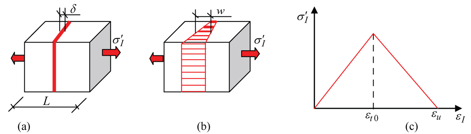
Figure 1: The Cohesive zone model of hydraulic....
The Cohesive zone model of hydraulic fracture: (a) The localized damaged band; (b) The cohesive breakdown process; (c) Relation between effective stress and strain.
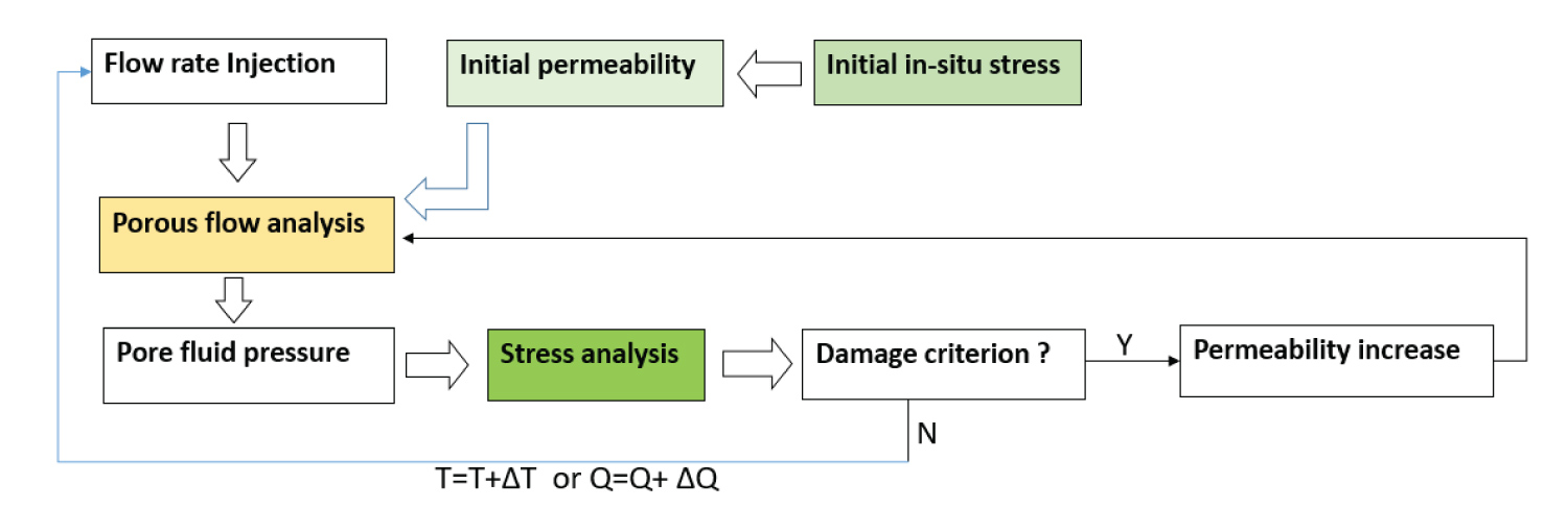
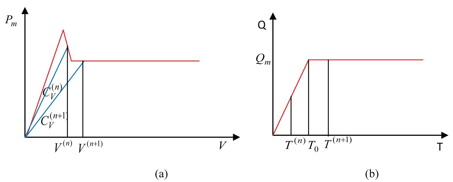
Figure 3: Loading Scheme of full flow....
Loading Scheme of full flow rate: (a) Relation of fluid pressure at crack mouth and loading flow rate; (b) Loading division of flow rate.
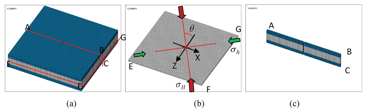
Figure 4: The 3-D FEM model (a), The horizontal....
The 3-D FEM model (a), The horizontal middle section (b) And vertical middle section (c)
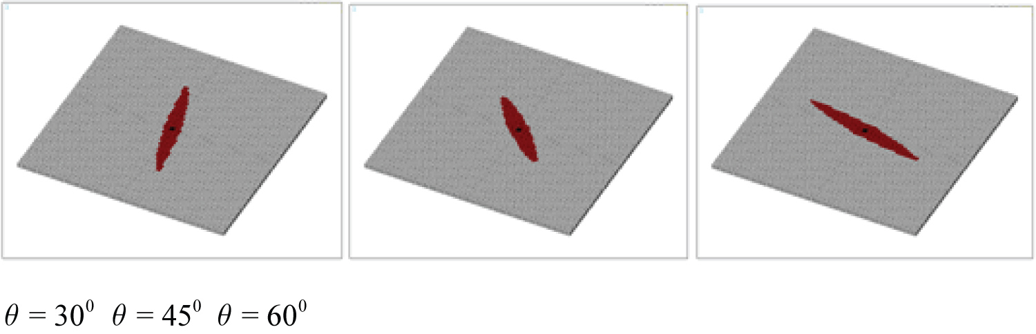
Figure 5: Hydraulic fracture propagation in the....
Hydraulic fracture propagation in the direction of maximum principal stress.
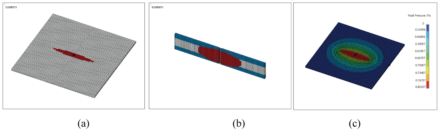
Figure 6: Horizontal middle section (a) Vertical....
Horizontal middle section (a) Vertical middle section (b) and Fluid pressure distribution (c)
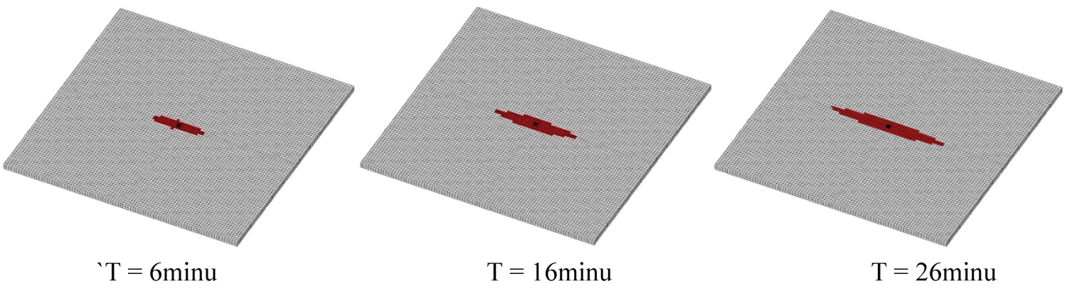
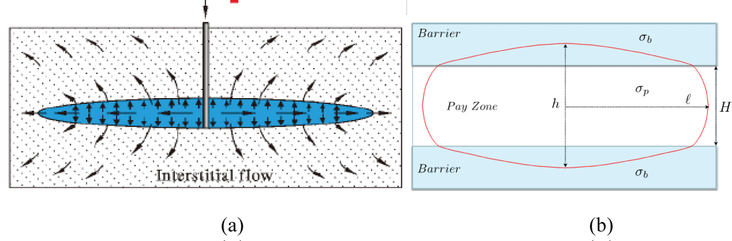
Figure 8: Coupling between Crack and porous...
Coupling between Crack and porous flow [30] (a) And the vertical outline of hydraulic fracture in three-layered formation [31] (b).
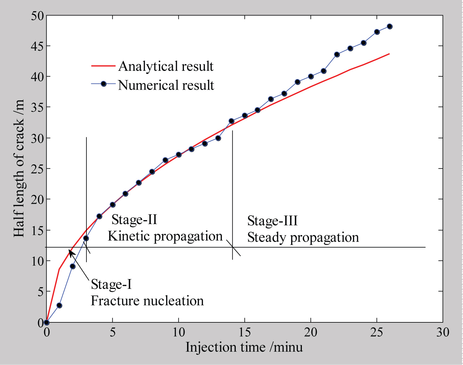
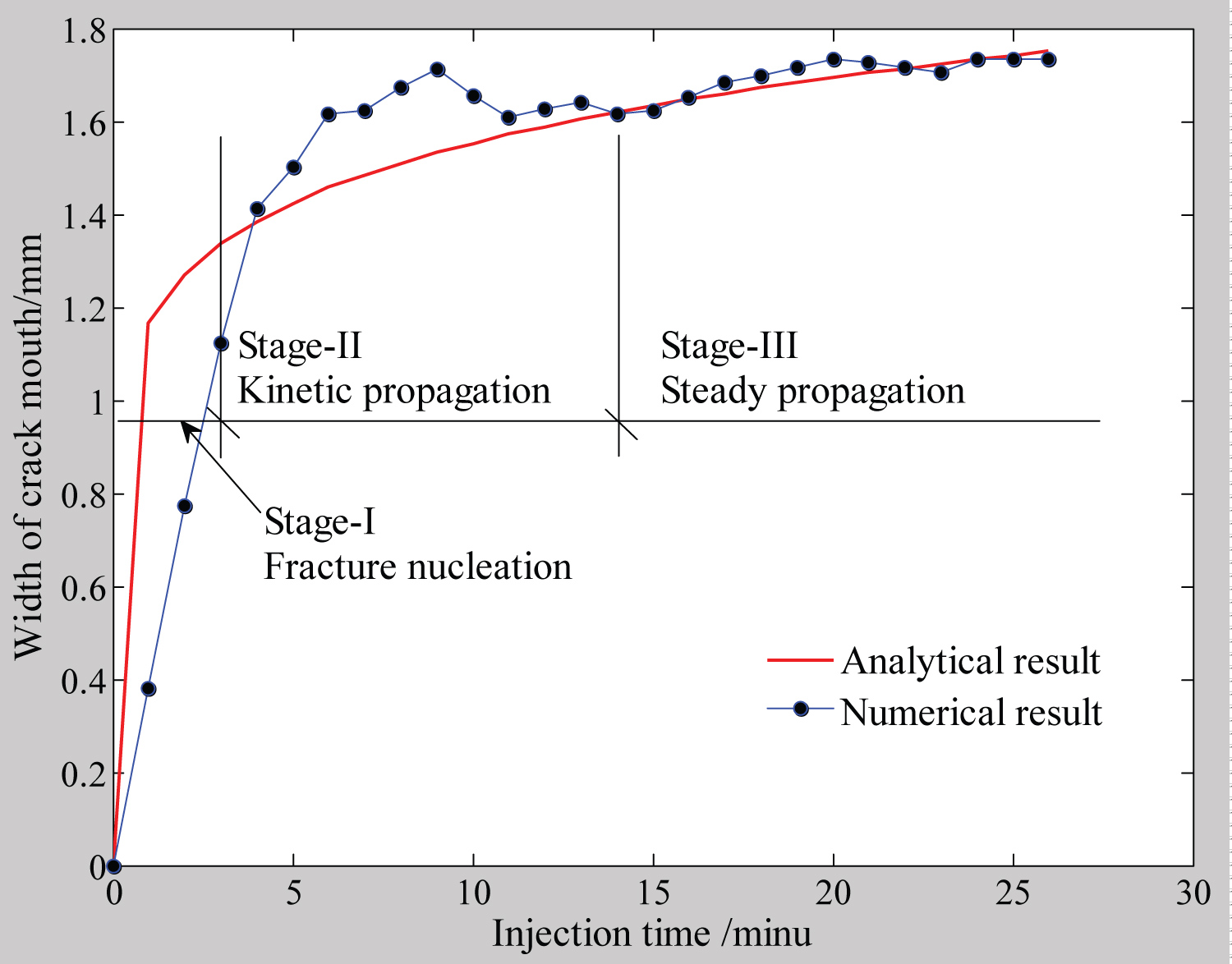

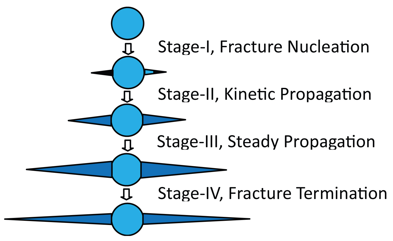
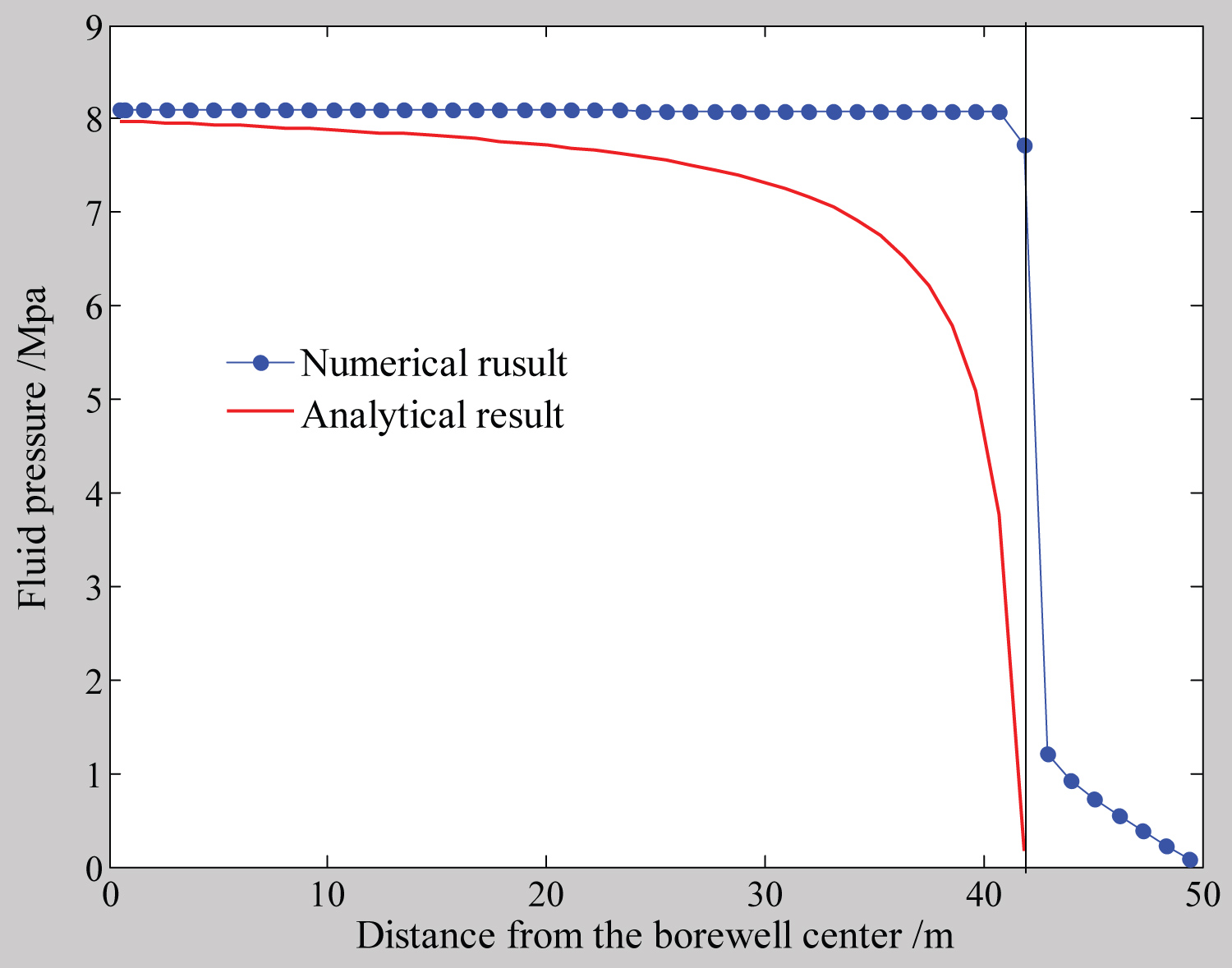
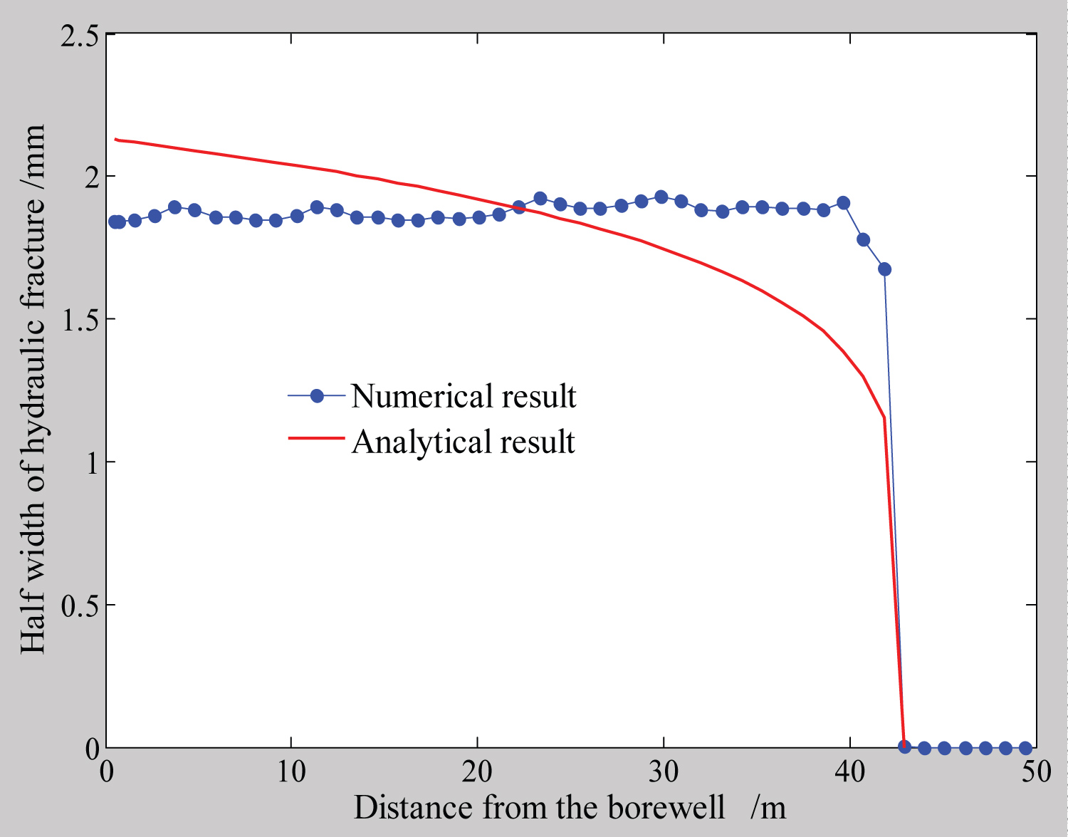
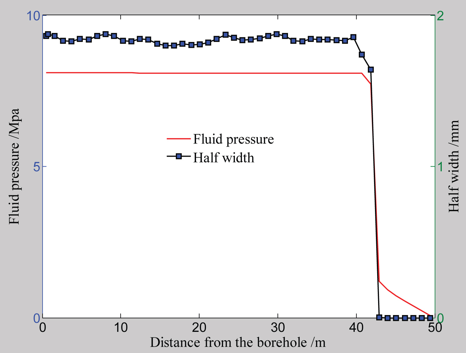
Figure 15: Contrast of numeric half width via....
Contrast of numeric half width via fluid pressure along fracture length.
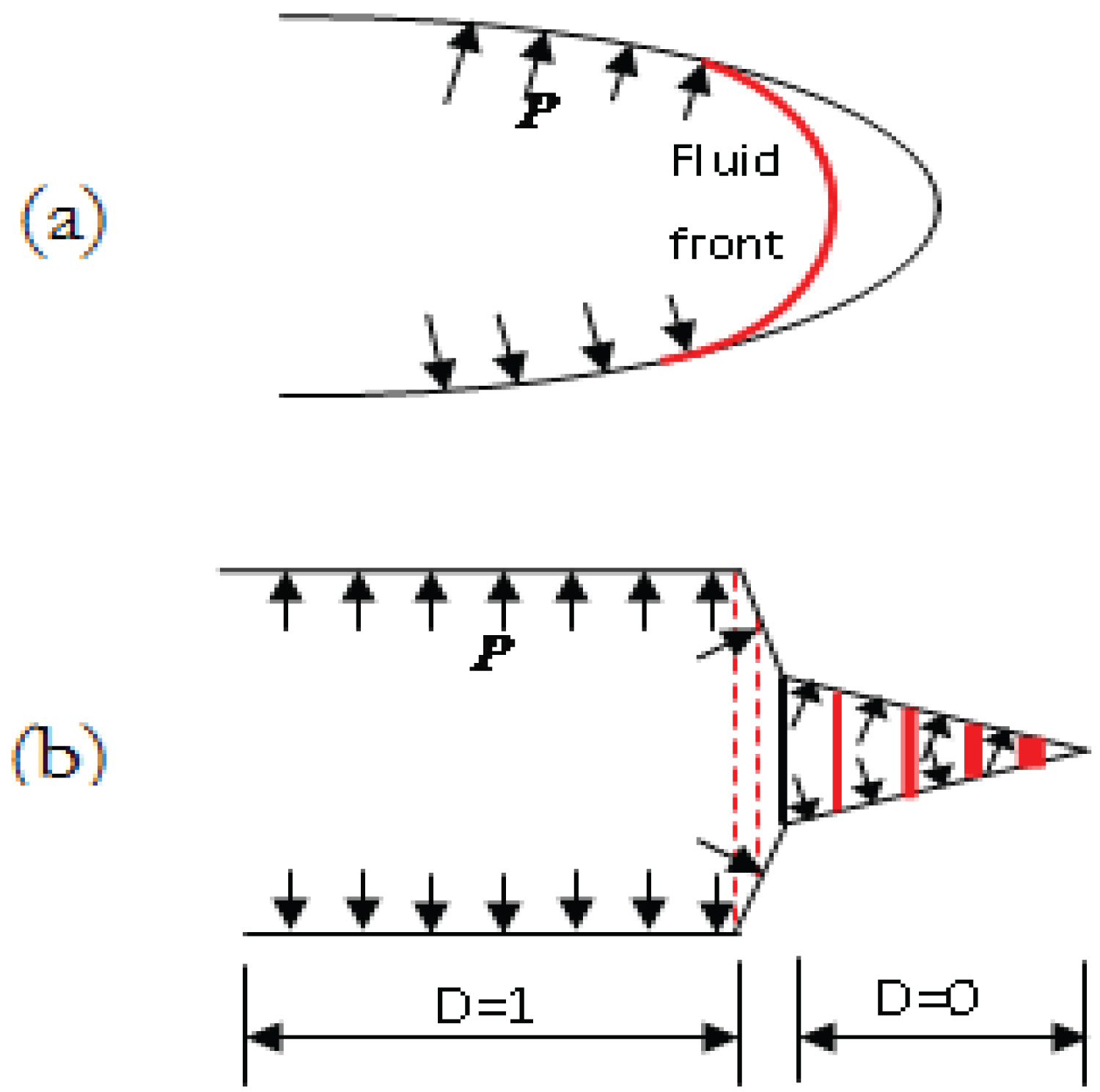
Figure 16: Coupling models: (a) Incomplete....
Coupling models: (a) Incomplete coupling model; (b) Complete coupling model.
References
- Perkins TK, Kern LR (1961) Widths of hydraulic fractures. J Pet Tech 13: 937-949.
- Nordren RP (1972) Propagation of a vertical hydraulic fracture. SPEJ 12: 306-314.
- Khristianovic SA, Zheltov YP (1995) Formation of vertical fractures by means of highly viscous liquid. Proceedings of the fourth world petroleum congress, Rome, 579-586.
- Greertsma J, de Klerk F (1969) A rapid method of predicting width and extent of hydraulically induced fractures. J Pet Tech 21: 1571-1581.
- Abe H, Mura T, Keer LM (1976) Growth-rate of a penny-shaped crack in hydraulic fracturing of rocks. Journal of Geophysical Research 81: 53335-53340.
- Settari A, Cleary MP (1986) Development and testing of a pseudo-three-dimensional model of hydraulic fracture geometry. SPE Trans AIME 281: 449-466.
- Morales RH (1989) Microcomputer analysis of hydraulic fracture behavior with a pseudo-three-dimensional simulator. SPEPE 2: 69-74.
- Clifton RJ, Abou-Sayed AS (1979) On the computation of the three-dimensional geometry of hydraulic fractures. SPE 7943.
- Barree RD (1983) A practial numerical simulator for three-dimensional fracture propagation in heterogenous media. Proceedings of the SPE Symposium Reservoir Simulation. San Francisco, California.
- Chen ZR, Bunger AP, Zhang X, Jeffrey RG (2009) Cohesive zone finite element-based modeling of hydraulic fractures. Acta Mechania Solid Sinica 22: 443-452.
- Zhang GM, Liu H, Zhang J, Biao F (2009) Simulation of hydraulic fracturing of oil well based on fluid-solid coupling equation and non-linear finite element. Acta Petrolei Sinica 30: 113-114.
- Wang H, Liu H, Zhang J, Wu H, Wang X (2011) Numerical simulation of hydraulic fracture height control with different parameters. Journal of University of Science and Technology of China 41: 820-825.
- Biao FJ, Liu H, Zhang SC, Zhang H (2011) A numerical study of parameter influences on horizontal hydraulic fracture. Engineering Mechanics 28: 228-236.
- http://www.ansys.com.
- Yang TH, Tang CA, Liang ZC, et al. (2003) Brittleness damage of rock failure process and seepage coupling numerical model study. Acta Mechanica Sinica 35: 533-541.
- Li LC, Liang ZC, Li G, Ma T (2010) Three-dimensional numerical analysis of traversing and twisted fractures in hydraulic fracturing. Chinese Journal of Rock Mechanics and Engineering 29: S3208-S3216.
- Lu YL, Elsworth D, Wang LG (2013) Microcrack-based coupled damage and flow modeling of fracturing evolution in permeability brittle rocks. Computers and Geotechnics 49: 226-244.
- Wang L, Ye JS, Mao YC, Yang JH, Rui DH (2013) Microcracks size growth prediction based on microdefects nucleation number. International Journal of Fracture 182: 239-249.
- Wang L, Mao YC, Ye JS, Yang JH, Rui DH (2013) Models for microcracks extension and damage evolution based on number series of microdefects nucleation. Engineering Mechanics 30: 278-286.
- Zimmerman RW (2000) Coupling in poroelasticity and thermoelasticity. International Journal of Rock Mechanics and Mining Sciences 37: 79-87.
- Kong XY (2000) Advanced poromechanics. Press of University of Science and Technology of China, Hefei, China.
- Bazant ZP, Oh BH (1983) Crack band theory for fracture of concrete. Materials and Structures 16: 155-177.
- Oda M, Takemura T, Aoki T (2002) Damage growth and permeability change in triaxial compression tests of Inada granite. Mechanics of Materials 34: 313-331.
- Zhou CB, Xiong WL (1996) Permeability tensor for jointed rock masses in coupled seepage and stress field. Chinese Journal of Rock Mechanics and Engineering 15: 338-344.
- Meng ZP, Zhang JC, Wang R (2011) In-situ stress, pore pressure and stress-dependent permeability in Southern Qin shui Basin. International Journal of Rock Mechanics & Mining Sciences 48: 122-131.
- Zimmerman RW, Bodvarsson GS (1994) Hydraulic conductivity of rock fractures. Earth Sciences Division, Lawrence Berkeley Laboratory, University of California, Berkeley.
- Witherspoon PA, Wang JSY, Iwai K, Gale JE (1980) Validity of cubic law for fluid flow in a deformable rock fracture. Water Resour Res 16: 1016-1024.
- Liu ZL, Wang T, Gao Y, Zhuang Z, Wang Y, et al. (2016) The key mechanics problems on hydraulic fracture in shale. Chinese Journal of Solid Mechanics 37: 34-38.
- Peirce A (2015) Modeling multi-scale processes in hydraulic fracture propagation using the implicit level set algorithm. Comput Methods Appl Mech Engrg 283: 881-908.
- Geertsma J, Haafkens R (1979) A comparison of the theories for predicting width and extent of vertical hydraulically induced fractures. J Energy Res Technol 101: 8-19.
- Zeng XH, Guo DL, Wang ZW, Zhao JZ (2005) Study on the calculating method of the total fracturing fluid leak-off coefficient. Journal of Southwest Petroleum Institute 27: 53-57.
- Adachi JI, Detournay E (2008) Plane strain propagation of a hydraulic fracture in a permeable rock. Engineering Fracture Mechanics 75: 4666-4694.
- Desroches J, Detournay E, Lenoach B, Papanastasiou P, Thiercelin M, et al. (1990) The crack tip region in hydraulic fracturing. Proc Soc London Ser A 447: 39-48.
- Peirce A (2010) A hermite cubic collocation scheme for plane strain hydraulic fractures. Computer Methods in Applied Mechanics and Engineering 199: 1949-1962.
Author Details
Wang Li1,2*, Guo Xiaohui1, Shi Bing2,3 and Cao Yunxing2,3
1Civil Engineering, Henan Polytechnic University, Jiaozuo, China
2Collaborative Innovation Center for Coalbed Methane and Shale Gas for Central Plains Economic Region, Jiaozuo, China
3Resources & Environment Institute, Henan Polytechnic University, Jiaozuo, China
Corresponding author
Wang Li, Civil Engineering, Henan Polytechnic University, Jiaozuo, China; Collaborative Innovation Center for Coalbed Methane and Shale Gas for Central Plains Economic Region, Jiaozuo, China.
Accepted: May 24, 2021 | Published Online: May 26, 2021
Citation: Li W, Xiaohui G, Bing S, Yunxing C (2021) Poromechanical Modeling of Hydraulic Fracture Propagation. Int J Earth Sci Geophys 7:046.
Copyright: © 2021 Li W, et al. This is an open-access article distributed under the terms of the Creative Commons Attribution License, which permits unrestricted use, distribution, and reproduction in any medium, provided the original author and source are credited.
Abstract
A poromechanical modeling of hydraulic fracture propagation is presented. It is established based on a constitutional model of fracture opening. Based on this constitutional model, a permeability tensor is established to model fracture propagation in different direction. Another is included into the computational equation. A full scheme of hydraulic fracturing simulation is presented in this paper.
Keywords
Hydraulic fracture, FEM, Poroelasticity, Damage, Fracture opening
Introduction
Hydraulic fracturing (HF) is an important technique in enhancing the permeability of petroleum and gas reservoirs. The mechanisms of fracture propagation are well understood by the analytical solutions (2D [1-5], P3D [6,7] and PL3D [8,9]) which are mainly dealing with the lubricant flow, elastic displacement of fracture walls and incomplete coupling between the fluid front and the fracture tip. However, the analytical solutions can only output temporal and spatial distribution of hydraulic fracture parameters such as fracture opening, length and fluid pressure on a predefined propagation path. Even some FEM methods [10-13] based on cohesive zone model also need to predefine the propagation path on lined nodes. These models ignore the temporal and spatial distribution of stress, damage, pore fluid pressure around the injection hole, which are significant in monitoring hydraulic fracture zone growth and assessment of permeability enhancement.
The poromechanical model can satisfy both the two needs for assessment of hydraulic fracture propagation. It is based on the coupling analysis between the porous flow and stress and damage utilizing the FEM, which is comprised of direct coupling and load transfer methods [14]. The former is also referred to as strongly coupled, where the final solution of the unknown multiple physical field variables are recovered by solving the simultaneous equations. However, many engineering problems do not satisfy the conditions of strong coupling, especially for some dynamical evolution problems such as damage-induced fracture - where it is difficult to ensure solution convergence. The load transfer method approaches a solution of the unknown field variables by successively solving the multi-physical field equations, during which one field variable is used as an input for the solution of another and repeated through the sequence of couplings until a tolerance for an equilibrium solution is reached. This load transfer, sequential, or leap-frog method represents only weak coupling, and since fluid-driven fractures are always evolving, hence this method is particularly appropriate for the nonlinearities in these problems. However, there are some key points in the poromechanical model to be dealt with, such as how to define the fracture opening using the continuum variables, how to deal with the strain energy loss resulting from hydraulic fracturing, how to control the direction of fracture propagation and how to apply the fluid load to simulate the continuum injection, etc. Previously, some hydraulic fracturing models [15-17] bypassed these issues.
In the present paper, we answer all these questions above. Basically, our poromechanical model is constituted of several components that (1) The fracturing opening is calculated based on damage localization employing a thickness of localization; (2) The strain energy loss resulting from fracturing is compensated by the fluid pressure invasion through poroelasticity coupling; (3) The direction of fracture propagation is controlled by the tensors of hydro-mechanical properties induced by hydraulic fracture opening; (4) The continuous injection with the fracture growth is achieved by a loading scheme of stepwise increased solution duration. As an example, the model is used representing hydraulic fracture propagation in a three-layer reservoir, the morphology of fracture zone and parameters such as length, width and fluid pressure are validated with the analytical solutions. And the model exhibits four stages of fracture propagation, which are fracture nucleation, kinetic propagation, steady propagation and propagation termination and represents the full coupling between fracture tip and fluid front.
Controlling Equations
We define the relations that enable the simulation of fluid-pressure effects on the propagation of a fluid-driven fracture. This involves both the transport of fluid and the mechanism of fracture expansion driven by that fluid.
Flow in porous media
In the reservoir formation, the porous flow satisfies Darcy' Law as
In which, P is pore fluid pressure, q is the velocity of fluid flow, is differential operator vector and K is the permeability, as,
From mass conservation, the pore pressure is determined as
Where is the mass of fluid, is fluid generation rate of a unit solid volume and t is time.
According to the coupling between the compressibility of the solid and fluid [18,19], the differential change of fluid mass, can be represented as
in which is the mass density of the fluid, is the differential increment of fluid mass, is the bulk volume and is the porosity. Eq. 4 shows that the volume increment of fluid comprises three parts in which and are the pore volume increment caused by the fluid pressure increment dP resulting from pore-elasticity and fluid compressibility, respectively, and is the compressive volume increment of the pore volume caused by an increment of the confining stress . The coefficient , represents the internal expansibility in volume resulting from the increment of fluid pressure, , the internal contractility in volume resulting from the increment of confining stress, and , the fluid compressibility resulting from increment of fluid pressure, they are defined as [20,21]
, , (5)
In which is the pore volume, is the average stress and the sign convention is with compression defined positive. Further, we can define the storage coefficient of fluid by adding the first and third expressions in Eq.5, as . Rewriting Eq. 4 and substituting this into Eq. 3, yields
This states that in any element of the porous media, the increment of fluid volume comprises three parts, the net increment that flow in minus flow out, source generation and drainage resulting from external stress increment, which are corresponding to the three terms in the right hand of this equation.
Stress rebalance
The pore fluid pressure will enlarge the longitudinal strains, so the total strain is the superposition of confining stress induced strain and pore pressure induced longitudinal strains, as that
In which is the total strain vector, is the (confining) stress vector, is an increment of pore fluid pressure, is the reference pore fluid pressure and is the linear expansion coefficient vector resulting from internal forces of fluid pressure increment. In the initial state is isotropic, , which is defined as
While is an bulk expansion coefficient, defined as [18,19]
By employing the concept of thermal elasticity, can also be calculated as
Where is the bulk modulus of the solid skeleton and is the Biot coefficient, thus
In which is the bulk modulus of matrix.
The stresses corresponding to the total strains in Eq. 7 are the effective stress , and can be written as
Since the pore fluid pressure is not uniformly distributed, so the effective stress will cause stress redistribution. The tensor form of the stress differential equation can be written as
Where is the body force per unit volume.
Fracture Opening and Anisotropy
As is mentioned previously, the key point using FEM to represent hydraulic fracture propagation is to establish the fracture opening in a continuum element, and based on this, to establish a series of second order Cartesian tensors of poromechanical properties such as damage, poro-elastic properties and permeability.
Fracture opening
Progressive fracturing in geo-materials transits a variety of scales and can be divided into three main stages: Evolution of distributed micro-damage, localization and subsequent macro-crack nucleation and macro-crack propagation [18,19,22]. For element of FEM, the entire fracture process can be represented by a damage variable and defined as
In this, is the threshold strain, representing the initiation of crack nucleation, is the final strain when the fracture has transected the porous element, and is a combined parameter, calculated as , and is the tensile strain controlling fracture opening. This tensile strain is in the same direction as the first effective principal stress (Figure 1), while the effective stress following the cohesive law (Figure 2).
The magnitude of the fracture opening can be determined from strain and damage, by employing the thickness of the damage localization band, which is noted as , typically 1-2 times the size of the cleat spacing. The element size is noted as L, thus it can be divided into two zones in the tensile direction: A concentrated damage zone of dimension and an undamaged zone of dimension . Both zones are subject to the same stress, , thus
Where w represents fracture opening, represents total elongation of the element and represents initial elastic modulus. From this equation, we have the relation
Since the total strain can be expressed as
Substituting Eq. 16 with 17 attains the hydraulic fracture opening, as
According to Eq. 7, the relation between strain and stress can be written as
Substituting Eq. 18 with Eq. 19, the constitutive relationship between fracture opening and fluid pressure is attained, thus
Where is the minimum confining stress normal to fracture surfaces, is taken as negative.
Fracture induced anisotropy
The presence of a hydraulic fracture will bring about anisotropy to the hydro-mechanical properties such as damage, coefficients of poroelasticity, and permeability. These may be represented using a series of second order Cartesian tensors, which are defined in the global coordinates.
Anisotropy of damage: The damage tensor in global coordinates can be converted from , which is defined in the coordinates of the principal stresses , as
Where is the conversion matrix, defined as
and
,
In this represents the tensile damage in the direction of , which is derived from Eq. 14. Hence, the damage tensor in global coordinates are written as
Anisotropy of poroelasticity coefficients: A hydraulic fracture also brings about anisotropy to the coefficients, and . For these a set of damage related coefficients are introduced to achieve the anisotropy, as that
and
In which and are the orthotropic coefficient vectors, with the components take the forms that
and , (26)
Here represents damage in the global directions of x, y, z.
Anisotropy of permeability: The permeability tensor resulting from a series of joints sets or fractures is well known [23,24]. However, all those only consider fluid flow along the fracture, neglecting the normal flow, which represents the leak-off. We established a permeability tensor considering the both flows, as that
In which K and are the matrix of permeability coefficients in global coordinates and principal stress coordinates, respectively, and is written as
In which , and are the three projections of the normal vector N of fracture surfaces on the three principal stress vectors; kn and are the normal and tangent permeability, respectively. The normal permeability kn can be recovered by modifying the in-situ permeability k with a modification , as
In which k is the in-situ permeability decreasing exponentially as the effective stress increases [25], calculated as
While is the intrinsic permeability tested in lab; is the effective average stress, noted as compression positive; is the reference stress, evaluated as the mean, maximum or minimum of magnitude vector of ; is a constant valued between 1.0 and 1.6.
The permeability along the fracture follows the cubic law [26,27] as
Here to all the components necessary for simulation of a hydraulic fracture propagation are established. In the next section, they are assembled by the weakly coupled FEM equations and run to work by the coupling analysis scheme.
Coupling Analysis
FEM format of coupling equations
The differential Eq. 6 and 13 can be transformed into FEM formats by utilizing Galerkin variational principle, so that in solid solution domain, the FEM format of Eq. 13 is written as
Where is the global stiffness matrix, a is the column matrix of the unknown nodal displacements, is the column matrix of solid load, is column matrix of fluid pressure, calculated as
Where D is the elasticity stiffness matrix of the porous rock, B is element strain matrix, is column matrix of incremental strain, generated by the incremental pore pressure .
In fluid solution domain, the FEM format of Eq. 6 can be written as
Where P is the column matrix of the unknown pore pressure, , is the permeability matrix; C is the matrix of storage coefficient, Q is the column matrix of flow rate, which are respectively assembled as
And
Where and are matrixes of poroelasticity assembled using the coefficients defined in Eq.5; , , are the column matrixes of flow rate, generation rate and confining stress change induced fluid content change, respectively. All the global matrixes are assembled as
, ,
While
,
, ,
In which N is shape function matrix. The weak coupling format of Eq. 32 and Eq. 34 is written as
Analysis process
As is showed in the analysis flow chart in Figure 2, the coupling analysis can be divided into several calculation parts:
(1) Establish in-situ stress and permeability. This is very important, especially if no perforation made. As is known that the in-situ permeability depends on the initial in-situ stress distribution with injection hole bored, while the distribution of permeability around the injection hole determine the positions where the fracture propagation initiates.
(2) Porous flow analysis. For which, the transient analysis is carried out with fluid flux as surface load, permeability as input and pore pressure as the output.
(3) Stress adjustment analysis. For which, the pore fluid pressure input as the body force, the strains and effective stresses are attained by statics solution.
(4) Damage judgment. If no more new damaged elements generated, increase injection flow rate or injection time, and repeats the processes above; Else, calculate fracture opening, anisotropy of hydro-mechanical properties, renew the input parameters and repeat the processes above. Goes on these, the numeric hydraulic fracture propagates.
Fluid loading scheme
In order to identify fracture growth during continuous injection, a loading scheme of a stepwise increased solution duration is adopted. This requires the assumption that the fracture can completely be closed when hydraulic fluid is drained so that the parameters of hydro-mechanical properties can be elastically handled. As is showed in Figure 3a, represents the global elasticity rigidness of surrounding rock, it decreases with the fracture propagation going on, while the increasing fluid loading is carried out by the increasing injection volume V. Based on this, the loading scheme is that keeping the flow rate constant, the fluid loading duration is stepped into small time steps, and for each transient analysis of flow, the solution duration stepwise increases with the input parameters kept renewed. Further, in order to simulate a real injection process, a limit flow rate Qm and a character time up to this pressure T0 are set up, hence the flow rate load Q at each transient analysis is written as
Correspondingly, the flux loaded on the walls of the injection hole through coal bed, is written as
where h represents coal bed thickness and d the hole diameter. In this paper
Example
FEM model
The example model (Figure 4) is taken from coal bed methane formation which is buried in 750 m depths, 200 m × 200 m in horizontal dimensions, 5 m thick for top and bottom beds, respectively, h = 10 m thick for coal bed, and d = 20 mm for injection hole diameter. The minor horizontal principal stress is , the major horizontal principal stress , with the stress ratio is . The vertical stress is calculated as , in which is mass density of overlaying rocks, H is buried depth, g is gravitational acceleration. All boundary displacements are set to zero, since it is the requirement of implanting initial stresses, and on the other hand, it is more reasonable for real in-situ deformation state. Figure 4a shows the formation compositions and positions of cross-sections, Figure 4b and Figure 4c show the middle horizontal and vertical sections with injection hole crossed. The direction of horizontal major principal stress is expressed using angle , which rotates anti-clockwise from negative Z coordinate. Following the in-situ.
Property parameters
The formation property parameters include permeability, coefficients of poroelasticity and damage model parameters. These are usually assumed satisfying Weibull distribution with the probability density function as
In which represents element property parameters, is the reference modulus, m is shape factor, representing the homogeneous degree of parameter distribution. The more m value is, the more uniform, in this paper, m = 10. The reference modulus are valued as in Table 1, which probably amount to their average values. Hydraulic fluid property parameters are listed in Table 2.
Results and validations
Hydraulic fracture zones: The numeric results of hydraulic fracture zone are shown in Figure 5, Figure 6 and Figure 7, from which the basic features can be derived, that
(1) Hydraulic fracture always propagates in the direction of the major principal stress , with the fracture surfaces normal to the minimum principal stress (Figure 5). This conforms to the routine knowledge and proves that the tensors established for the hydromechanical properties are right and can effectively control the direction of fracture propagation.
(2) The horizontal cross-section of fracture zone and fluid pressure contours are approximate to ellipse areas. This conforms to that computed by Liu [28] (Figure 8a) and those described in [1-13].
(3) The vertical section is approximate to an ellipse area, and slightly cut through the top and bottom beds in the vicinity of injection hole (Figure 6b). This conforms to that proposed by Peirce [29] for three-layered formation (Figure 8b).
Temporal variation of hydraulic fracture parameters: The parameters of hydraulic fracture include fracture length, opening and fluid pressure. The fracture lengths are measured from the resultant pictures in Figure 7. The fracture openings and fluid pressure at fracture mouth are measured by setting a monitor element at fracture mouth for every transient analysis. The comparisons of the temporal variation of these parameters via the analytical solutions are showed in Figure 9, Figure 10 and Figure 11. The analytical solutions proposed by Nordgren [2], Geertsman & Klerk [30] for KGD and PKN models in the case of high leak-off, are adopted, hence
Where G is coal bed shear constant, S is the principal stress normal to fracture surfaces, , represents the effects of leak-off, , is leak-off coefficient involving with permeability, porosity, in-situ stresses, fracture toughness and fluid viscosity, etc, is valued as [31], and is injection flux.
The comparisons show that numeric solutions are well conformed to the analytical solutions, while some slight differences indicate that the numeric solutions can exhibit more plentiful information about hydraulic fracture propagation. Base on these differences the process of hydraulic fracturing can be divided into four stages, which are conceptualized in Figure 12, that
Stage-I, fracture nucleation, during which, a macro embryo fracture takes its form in the close vicinity of injection hole. Since it is aggregated from distributive cracks, the gaps and bridging of them constitute fracture cohesive zones. In this stage the peak fluid pressure is used both in overcoming the traction of cohesive zone and support the confining normal stress;
Stage-II, kinetic propagation, during which, the sudden break of cohesive traction causes that the fluid pressure at fracture mouth has a big drop, the fracture opening goes fast up to a peak value and fracture length increases fast. These indicate a kinetic propagation.
Stage-III, steady propagation, during which, the fluid pressure at fracture mouth keeps constant while fracture length goes up fast and fracture opening goes to a constant slowly.
Stage-IV, propagation termination, during which, as fracture length increases, the injection flow rate cannot afford to going up of leak-off, so that gives rise to slow drop of fluid pressure, decrease of fracture opening and propagation termination in the end.
It is obvious that the analytical solutions ignore stage-I and stage-IV.
Spatial variation of parameters of hydraulic fracture: The analytical solutions of fracture opening and fluid pressure along fracture length are the so-called SCR asymptote by Adachi & Detournay, et al. [32-34], as that
In which are the dimensionless forms of fracture opening, fluid pressure, position coordinate, fracture length, injection time and viscosity scaling, respectively. The comparisons between numerical solutions and the analytical solutions for fluid pressure and half width along the fracture length are showed in Figure 13 and Figure 14. The contrast between fluid pressure and half width along the fracture length is showed in Figure 15.
The comparison in Figure 13 shows that fluid pressure goes head of fracture tip and is almost evenly distributed along fracture hull. This is somewhat different from the analytical solutions. However, if we realize the premise of analytical solution, we would like to accept the numeric solution. Since mathematical difficulties, in analytical solutions the coupling between fracture tip and fluid front is generally assumed to be progressive, so that the fluid pressure distribution is always lagged behind fracture tip and that a pressure void always exists ahead of fluid front. So we can regard the analytical solution as the case of incomplete coupling between fracture tip and fluid front, which always occurs in the situations of large toughness, high viscosity and no leak-off; while in most cases, fluid pressure distribution goes ahead of fracture tip, complete coupling occurs, this is the case that numeric solution represents. The comparisons in Figure 14 and Figure 15 further indicate that there is cohesive zone ahead of the fracture tip.
Based on these, we can give out two types of coupling modes in fracture tip, the incomplete coupling model (Figure 16a) and complete coupling model (Figure 16b), which are corresponding to the analytical models and numeric solution in present paper, respectively. In the complete coupling model, D = 1 represents completely fractured zone, D = 0 represents elastically expansion zone of pore pressure, in between them, 1 > D > 0 represents cohesive fracture zone, the fracture opening is more like an aequilate 'bag', indicating that fluid pressure energy are mainly used in overcoming in-situ stress clamping and viscosity dissipation from fluid front invasion and leak-off.
Summary
In this paper we systematically clarified poromechanical modeling of hydraulic fracture propagation, which is proved to be correct and effectively. Especially, it is of the advantage that can be used in simulation of hydraulic fracturing in complex stress and inclined formation, which is the main aim we work to. Also some limitations should be noted here, that
(1) The fracture criterion and opening calculation method cannot be simply generalized to incomplete coupling model, in which case the toughness, viscosity and low leak-off are large,
(2) The thickness of localized fracture band is a material parameter, should be a specifically researched, and
(3) The patterned fracture zone shows that hydraulic fracture is not mere a plane but a band zone. This is verified by micro seismics monitored on the spot. Of course, the precision of fracture zone is element size related, it should not be larger than the size of RVE.
Acknowledgements
Many thanks to Special project for the 13th five-year plan, China, the project number is 2016ZX05067006-002.