
International Journal of Magnetics and Electromagnetism
(ISSN: 2631-5068)
Volume 7, Issue 1
Research Article
DOI: 10.35840/2631-5068/6536

Article Formats
Inversion of Magnetic Measurements of the Swarm A Satellite of the Bangui Magnetic Anomaly
Table of Content
Figures

Figure 1: The figure maps the border of....
The figure maps the border of the African counties, the Central African Republic is indicated.
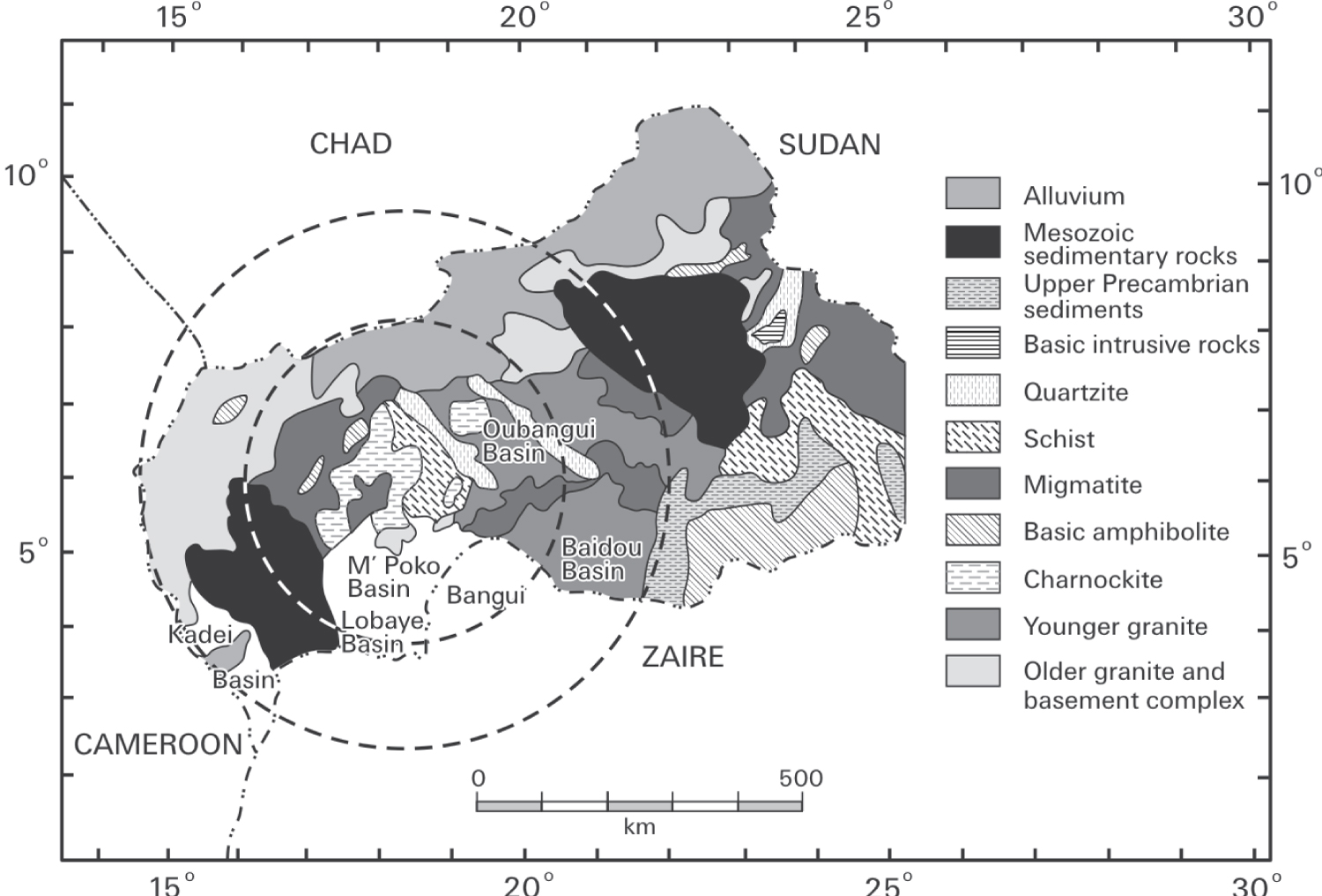
Figure 2: Simplified geological map in the.....
Simplified geological map in the region of the Bangui magnetic anomaly in the Central African Republic. The double circles show (later discussed) the position of the impact structure (Girdler, et al. [13]).
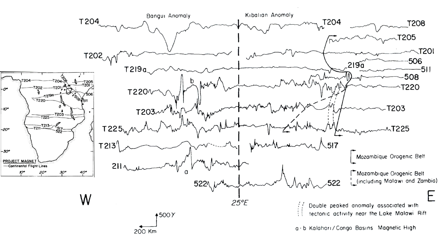
Figure 3: Bangui magnetic anomaly at 3 km....
Bangui magnetic anomaly at 3 km altitude. Several profiles are presented with Profile T 204 showing the Bangui total magnetic anomaly. The position of the flight lines is shown in the left side (Green [9]).
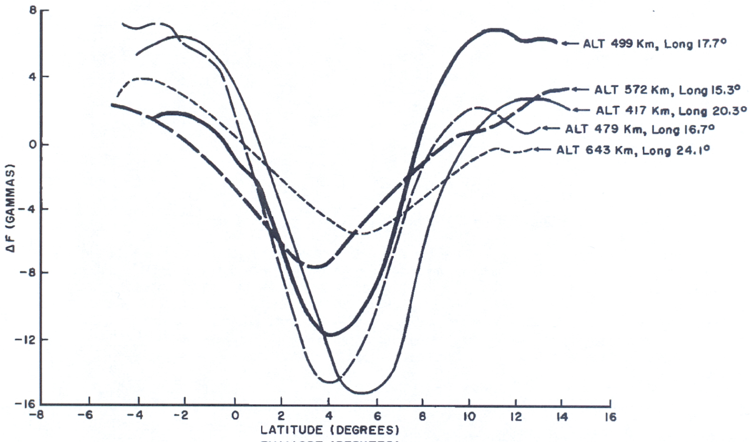
Figure 4: Magsat data indicating the Bangui....
Magsat data indicating the Bangui magnetic anomaly at different altitudes and longitudes (Regan and Marsh [11]).
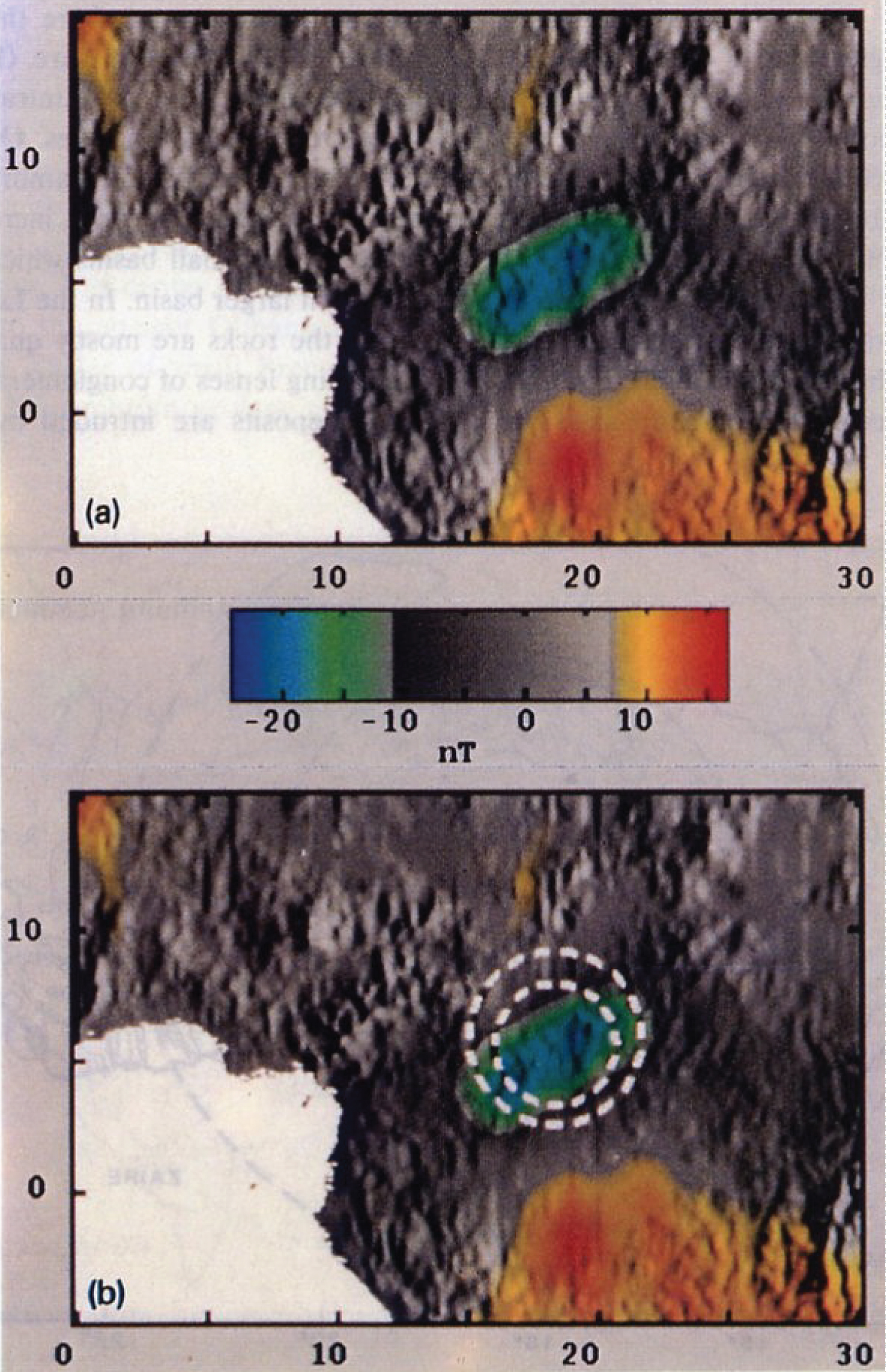
Figure 5: The Bangui Magsat magnetic anomaly....
The Bangui Magsat magnetic anomaly superimposed on a topographic image (upper), the Bangui Magsat anomaly map superimposed on the topographic image with the double ring structure (lower) (Girdler, et al. [13]).

Figure 6: Bangui total magnetic anomaly plotted....
Bangui total magnetic anomaly plotted on a Transverse Mercator projection.
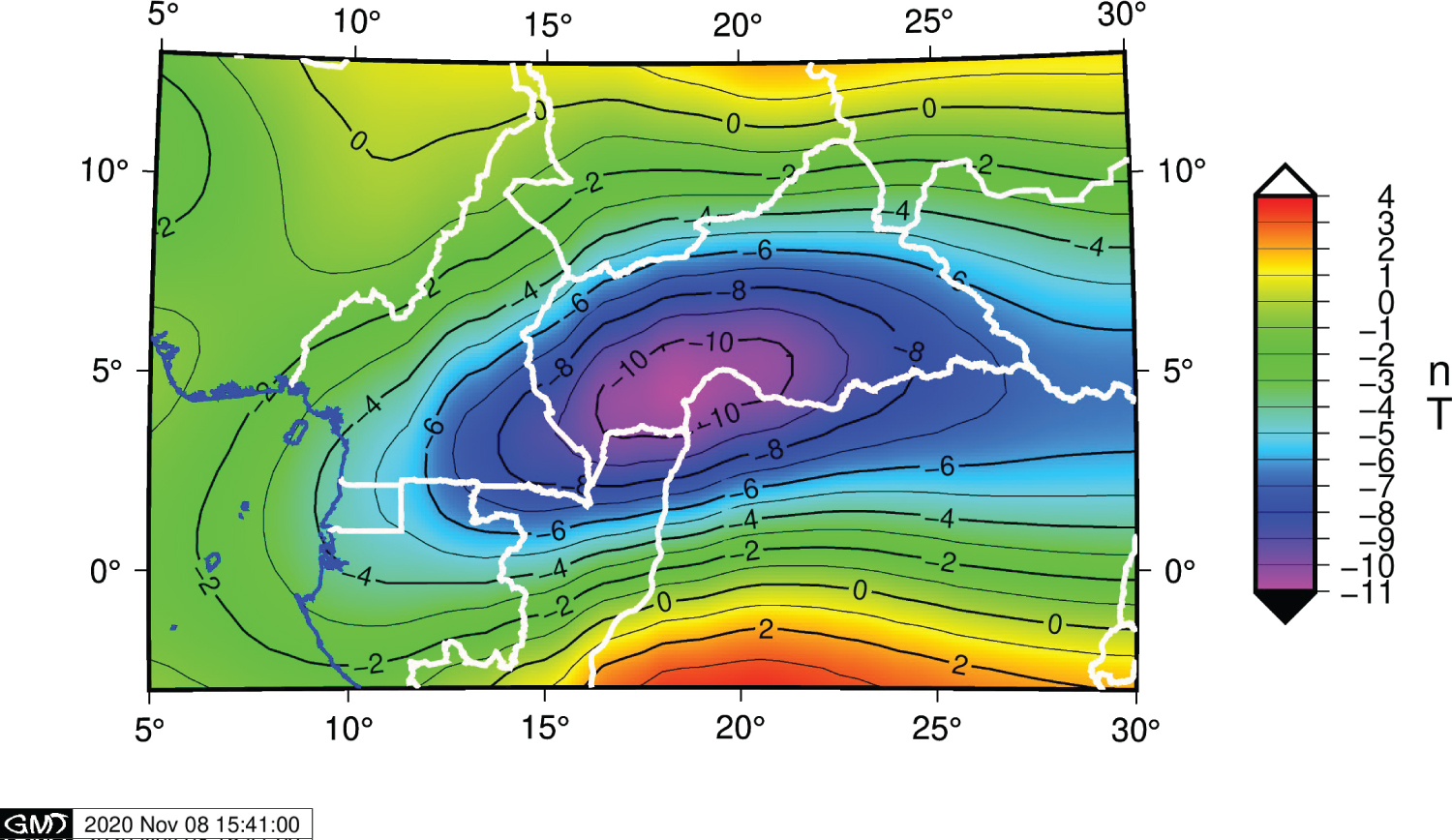
Figure 7: Reduced extension Bangui total magnetic...
Reduced extension Bangui total magnetic anomaly applied for the inversion procedure, the anomaly is plotted on a Transverse Mercator projection.
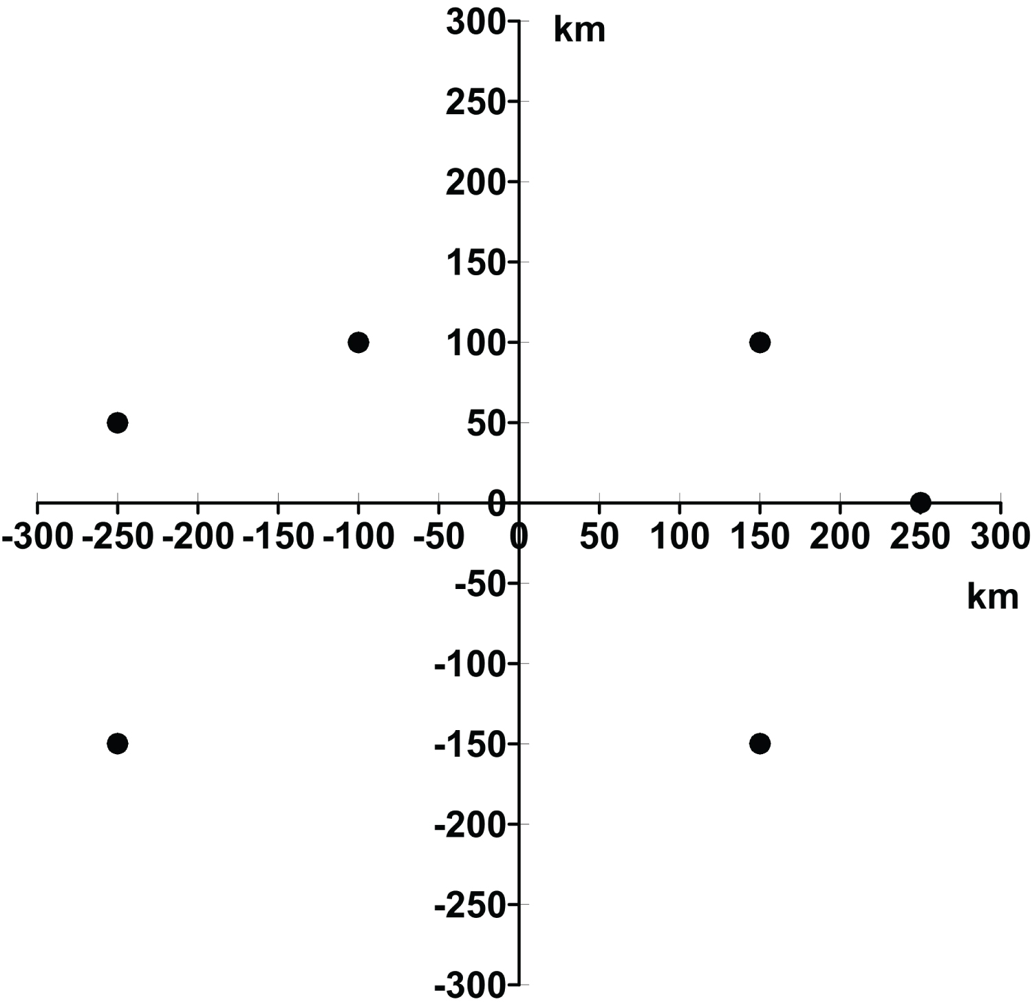
Figure 8: The horizontal coordinates...
The horizontal coordinates of the applied points of forward problem are plotted in Descartes coordinate system. The origin of the Descartes coordinate system is positioned in the point of (polar distance) θ = 86° and (longitude) λ = 19°.
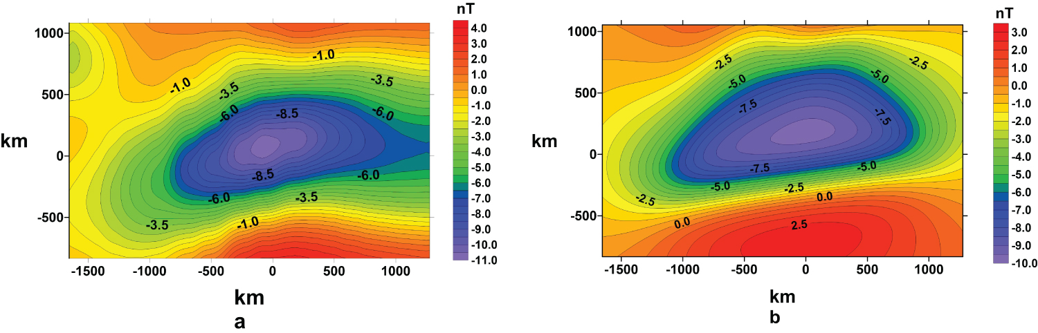
Figure 9: The reduced extension of the...
The reduced extension of the Bangui total magnetic anomaly (the input of the inversion): a) And the anomaly map determined by the inversion; b) The anomalies are plotted in the Descartes coordinate system. The origin of the Descartes coordinate system is positioned in the point of (polar distance) θ = 86° and (longitude) λ = 19°.
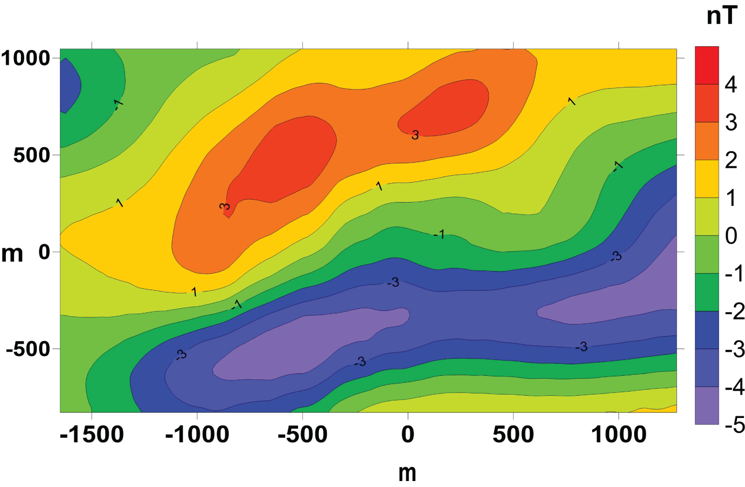
Figure 10: The difference between the input...
The difference between the input Bangui anomaly and the anomaly determined by inversion.
References
- Langel RA, Hinze WJ (1998) The magnetic field of the Earth's lithosphere. Cambridge University Press.
- Taylor PT, Schnetzler CC, Regan RD (1989) Satellite magnetic data: How useful in exploration? The Leading Edge 8: 26-28.
- Taylor PT, Schnetzler CC (1990) Satellite magnetic data: The exploration industry rates their usefulness. The Leading Edge 9: 42-43.
- Kis KI, Taylor PT, Wittmann G, Toronyi B, Puszta S (2011) Inversion of magnetic measurements of the CHAMP satellite over the Pannonian Basin. Journal of Applied Geophysics 75: 412-415.
- Taylor PT, Kis KI, Toronyi B, Puszta S, Wittmann G (2019) Interpretation of the magnetic measurements of the Swarm A over Central Europe. International Journal of Astronautics and Aeronautical Engineering 4: 29.
- Kis KI, Taylor PT, Wittmann G (2016) Determination of the Earth's magnetic field gradients from satellite measurements and their inversion over Kursk magnetic anomaly. International Journal of Astronautics and Aeronautical Engineering 5: 1000164.
- Taylor PT, Kis KI, Wittmann G (2013) Interpretation of CHAMP magnetic anomaly over the Pannonian Basin region using lower altitude gradient data. Acta Geodaetica et Geophysica 48: 275-280.
- Godivier R, LeDonche L (1956) Réseau magnétique remené au 1re Janvier 1956. République Centafricain Thad Méridional, Office de la Rech. Sci. et Techo, Outre-Mer, Paris.
- Green AG (1976) Interpretation of project magnet aeromagnetic profiles across Africa. Geophysical Journal of the Royal Astronomical Society 44: 203-228.
- Hastings DA (1982) Preliminary correlations of Magsat anomalies with the tectonic features of Africa. Geophysical Research Letters 9: 303-306.
- Reagan RD, Marsh BD (1982) The Bangui magnetic anomaly: Its geological origin. Journal of Geophysical Research 80 B2: 1107-1120.
- Ravat DN (1989) Magsat investigations over the greater African region. PhD Thesis, Purde University.
- Girdler RW, Taylor PT, Frawley JJ (1993) A possible impact origin for Bangui magnetic anomaly (Central Africa). Tectonophysics 201: 45-58.
- Grieve RAF (1987) Terrestrial impact structures. Ann Rev Earth Planet Sci 15: 245-270.
- Taylor PT (2007) Bangui anomaly. Encyclopedia of Geomagnetism and Paleomagnetism, 39-40.
- Kim HR (2007) CHAMP satellite magnetic anomaly map. Encyclopedia Geomagnetism and Paleomagnetism, 1002.
- Ouabego M, Quesnel Y, Rochette P, Demory F, Fozing EM, et al. (2013) Rock magnetic investigation of possible sources of the Bangui magnetic anomaly. Physics of the Earth and Planetary Interiors 224: 11-20.
- Tchoukeu CDN, Basseka CA, Djomani YP, Rousse S, Etame J, et al. (2021) Crustal thickness, depth to the bottom of magnetic sources and thermal structure of the crust from Cameroon to Central African Republic: Preliminary results for a better understanding of the origin of the Bangui Magnetic Anomaly. Journal of African Earth Sciences 179: 104206.
- Leger JM, Jager T, Bertrand F, Hulot G, Brocco L, et al. (2015) In-flight performance of the Absolut Scalar Magnetometer vector mode on board the Swarm satellites. Earth, Planets and Space 67: 57.
- Thébault E, Finlay CHC, Beggan CD, Alken P, Aubert J, et al. (2015) International Geomagnetic Reference Field: The 12th generation. Earth Planets and Space 67: 79.
- Plouff D (1976) Gravity and magnetic fields of polygonal prisms and application to magnetic terrain corrections. Geophysics 41: 727-741.
- Box GEP, Tiao GC (1973) Bayesian Inference in Statistical Analysis. International Statistical Review 43: 242-243.
- Tarantola A (1987) Inverse problem theory: Methods for data fitting and model parameter estimation. Elsevier, Amsterdam, Oxford, New York, Tokyo.
- Duijndam AJW (1988) Bayesian estimation in seismic inversion part I: Principles. Geophysical Prospecting 36: 878-898.
- Duijndam AJW (1988) Bayesian estimation in seismic inversion part II: Uncertainty analysis. Geophysical Prospecting 36: 899-918.
- Menke W (1989) Geophysical data analysis: Discrete inverse theory. Academic Press, Inc. San Diego, New York, Boston, Sydney, Tokyo, Toronto.
- Gregory PC (2005) Bayesian logical data analysis for the physical sciences. Cambridge University Press.
- Walsh GR (1975) Methods of optimization. John Wiley & Sons, London, New York, Sydney, Toronto 82: 200.
- Clifford AA (1973) Multivariate error analysis: A handbook of error propagation and calculation in many-parameter systems. Applied Science Publishers, London.
Author Details
KI Kis1*, PT Taylor2, B Toronyi3 and S Puszta4
1Geophysics and Space Science Department, Loránd Eötvös University, Hungary
2Geodesy and Geophysics Laboratory NASA/GSFC Greenbelt, USA
3Department of Geodesy and Surveying, Budapest University of Technology and Economics, Hungary
4Fractal Partnership, Hungary
Corresponding author
KI Kis, Geophysics and Space Science Department, Loránd Eötvös University, 1117 Budapest, Pázmány Péter sétány 1/c, Hungary.
Accepted: August 07, 2021 | Published Online: August 09, 2021
Citation: Kis KI, Taylor PT, Toronyi B, Puszta S (2021) Inversion of Magnetic Measurements of the Swarm A Satellite of the Bangui Magnetic Anomaly. Int J Magnetics Electromagnetism 7:036.
Copyright: © 2021 Kis KI, et al. This is an open-access article distributed under the terms of the Creative Commons Attribution License, which permits unrestricted use, distribution, and reproduction in any medium, provided the original author and source are credited.
Abstract
We wanted to make a satellite altitude magnetic anomaly map of the large magnetic anomaly in the Central African Republic, the Bangui magnetic anomaly, with data from the Swarm satellites. In the first part of our study, we summarize the earlier investigations and their interpretation. In the second we discuss our data processing applied to produce a magnetic anomaly map. We used the IGRF 12th to remove the long-wavelength regional anomalies. We will use an inverse procedure, which always requires a solution of the direct problem, and a horizontal polygonal prism given in the Descartes coordinate system. For this, reason the total magnetic anomaly was transformed into the Descartes coordinate system. The magnetization and its direction were used from our previous paper. The inverse problem is solved by the Simplex procedure. Our selected polygon has 14 geometrical parameters however, the inverse problem that is the numerical determination of the minimum problem is solved in the 14 dimensions. The result of our inverse problem was the 12 horizontal coordinates and the two upper and lower data of the polygon. The origin of the Bangui anomaly has been discussed in several scientific reports, either as a deep crustal tectonic feature or the result of a large external impactor. However, according to our inversion computations we cannot make any unambiguous finding for the origin of this feature. The inaccuracy in our total anomaly map is given by the Gaussian error propagation.
Keywords
Swarm A satellite, Bangui total magnetic anomaly, Optimization
Introduction
Satellite altitude magnetic measurements originate in the crust. The interpretation of these data has a longer history. They started with data from Cosmos, POGOs, Magsat, Oersted, CHAMP and SAC-C satellites. A summary of these satellites is given by Langel and Hincze [1]. The recent SWARM satellites provide more data.
In earlier papers by Taylor, et al. [2], Taylor and Schnetzler [3] they drew the attention to the application of satellite anomalies for resource exploration. They suggested the appropriate altitude, the required accuracy, and errors of these measurements.
We have made several geologic/tectonic interpreted of satellite magnetic anomalies see [4-7].
Bangui magnetic anomaly
The Bangui magnetic anomaly is located slightly north of Bangui city in the Central African Republic (Figure 1). The anomaly is near 6°N, 18°E and is one of the largest anomalies on Earth.
This magnetic anomaly was located by ground magnetic measurements by ORSTOM (Office de la Recherche Scientifique et Technique Outre-Mer) in 1953 by Godivier and Le Donche [8]. This magnetic anomaly is located in the Precambrian shield and it borders Oubangui, Lobaye basins and some sub-basins. The rocks are migmatites, charnockites, metadiabases and metasedimetary (Figure 2).
One of the airborne magnetic profiles (No. T-204) recorded by Project Magnet [9] at 3 km altitude crosses this anomaly. Green [9] found a negative anomaly of -1500 nT (Figure 3). According to his interpretation an impact by an iron meteor is the cause of this negative magnetic anomaly.
Hastings [10] presented a preliminary interpretation Magsat data of Africa. He interpreted the Bangui magnetic anomaly as an uplift of the Precambrian shield. The nearly horizontally magnetized source produces the central negative anomaly.
Regan and Marsh [11] interpreted this anomaly as an intrusion of a large mafic pluton into the crust. They presented the anomalies measured in different altitudes and latitudes (Figure 4). This intrusion is isostatically compensated because it is warped down into the crust. This negative Bouguer anomaly is caused by the sedimentary rocks filling the basin. The causative body ranges the depth from 3 km to 35 km. Its magnetic susceptibility is 0.01 (SI), and the density contrast is 100 kgm-3. The sedimentary rocks which cover the intrusive body has a susceptibility of 10-6 (SI) and a density contrast of -150 kgm-3.
Ravat [12] interpretated this magnetic anomaly to be created by an Fe-Ni-rich meteorite or Fe-rich iron formation.
Girdler, et al. [13] presented the LANDSAT topographic image and the Magsat magnetic anomaly superimposed on the topographic image (Figure 5). This image reveals a double ring structure with the outer ring diameter of 810 km and the inner ring diameter of 491 km. The larger diameter of the outer ring suggests that the impact was a very large body whose diameter could be of the order of 80-200 km. If this structure is caused by an early Precambrian impact it is the largest crater on the Earth's surface. One hundred and twenty terrestrial impact structures have been recorded (Grieve [14]). Gridler, et al. [13] interpreted the anomaly by a simple disk model with a diameter of 800 km and a thickness of 4.5 km. The top of this depth of 3 km. The magnetization is assumed to be 10 Am-1 and its direction is D = 18° and I = 25° respectively. The direction of the inducing field is D = -3° and I = -12°, and κ = 0.63 (SI) respectively. These values were used in the inversion calculations. The negative Bouguer anomaly was the result of the sediment covering the impact structure which has a lower density.
Several (Taylor [15], Kim [16]) have investigated the Bangui magnetic anomaly from the CHAMP magnetic measurements.
Ouabego, et al. [17] investigated the distribution of magnetic rocks to determine the cause of the Bangui magnetic anomaly. According to their investigation they do not find an impact as the source of this anomaly. Their interpretation of the source of this anomaly is the African plate interacted with the old cratons of the Gondwana land, with the anomaly probably the result of the Neoproterozoic iron rich metasediments.
Tchoukeu, et al. [18] investigate the Bangui magnetic anomaly and surrounding geological structures. They conclude that the source of the anomaly is of a crustal origin.
Data Processing
The SWARM satellites were launched from the Plesetsk cosmodrome on November 22, 2013 it is operated by the European Space Agency under the Living Planets Program.
The Swarm satellites were launched with nearly circular orbits. Two of them (A and C) orbit in tandem with an initial altitude of 460 km, while the initial altitude of the third satellite (B) is 530 km. The inclination of the A and C satellites is 87.4° while the satellite B has an 88° inclination. A and C satellites have their orbit nearly parallel with their approximate spherical separation of 1.5° at the Equator.
We mapped Swarms A's data between February 27, 2015 and July 20, 2015.
The Swarm satellites have flux-gate vector magnetometers and Overhauser scalar magnetometer [19], they record the field every second. Each day there are 86,400 data records. Since one period of revolution is ca. 90 minutes, one day registration (one file) includes 16 satellite revolutions.
The magnetic measurements of the SWARM satellites can be found in the ESA Level 1B folder. These data are given in CDF (Content Definition File) format.
First, we convert the CDF format to the ASCII (American Standard Code) with a public Matlab program.
Our downloaded files contained: date and time of the measurements, spherical coordinates (latitude, longitude, and spherical radius); X, Y, Z components; and the total magnetic field with their measurements errors are selected for further calculations.
Data were selected when the Kp index was less than 2+ . The Kp index are given by the IAGA International Service of Geomagnetic Indices (https://www.gfz-potsdam.de/en/kp-index).
The next step of the data processing is the determination of the anomalies. The reference level of the anomalies is determined by the 12th generation of the International Geomagnetic Reference Field [20]. Susan Macmillan (British Geological Survey) wrote a FORTRAN program for the calculation of the IGRF which is in home page of the IAGA (https://www.ngdc.noaa/IAGA/vmod/igrf13.f). The reference field can be calculated for the time and position of the measured satellite data. This program is used to determinate the ∆X, ∆Y, ∆Z and ∆T anomalies. These components are determined for the entire orbit.
The anomalies were selected for our research area. The limits of spherical quadrangle which covers the Bangui research area are, latitude -9.75° ≤ φ ≤ 19.25° and longitude 0.25° ≤ λ ≤ 29.5°.
Determination of the Bangui total magnetic anomaly
The appropriate satellite data are separated into downward and upward orbits. These orbits show approximately North and South directions. A median filter is applied for the eliminations of the outlier measurements. After this procedure, a different degree of polynomials was fitted to the separate downward and upward orbits. Because the linear trends are dominant, they were subtracted from the downward and upward orbits. Since the appropriate orbits show a similar character their means are processed for the further calculations. In the last step a low-pass filter was applied. This the low-pass filter was selected for calculating the dipole field at 460 km altitude. The resulting total anomaly field of our research is given in Figure 6. It is on a Transverse Mercator projection and the inversion procedure, a reduced size of the total anomaly field is applied (in latitude -3° ≤ φ ≤ 13° and longitude 5° ≤ λ ≤ 29.5°). The reduced size anomaly field is shown on a Transverse Mercator projection (Figure 7).
It is often required to transform satellite data from spherical polar coordinates to Cartesian the xyz coordinate system. This procedure is applied see [4]. The transformation can be done in two steps: A translation and a rotation.
Forward problem
The basic idea of the inversion is the selection an appropriate forward problem. The inversion always determines the parameters of the model of the forward problem. Among several possibilities the Plouff's [21] model is applied as a solution to the forward problem. His polygonal prism model has a horizontal top (z1) and bottom (z2) faces.
The total magnetic field of the polygonal prism is given by the equation:
Where μ0 is the permeability of a vacuum, Jx, Jy and Jz are the magnetic components of the anomalous body, l, m and n are direction cosines of the Earth's magnetic field:
l = cos I cos D , m = cos I sin D and n = sin I,. (2)
In the previous equations D and I are the declination and inclination of the Earth's magnetic field, respectively, V1, ... V6 are the volume integrals determined by the polygonal prism.
Ignoring the effects of demagnetization, the components of the total magnetization vector are
Where κ is the magnetic volume susceptibility, T is the magnitude of the Earth's magnetic field in the vicinity of the body, the L, M and N are the direction cosines of the remanent magnetization, Jr is the intensity of remanent magnetization.
The direction cosines of the remanent magnetization are determined by the following:
L = cos α cos β , M = cos α sin β , N = sin α (6)
α and β are the inclination and declination of the remanent magnetization, respectively.
According to Girdler, at al. [13] the remanent magnetization is assumed to be 10 Am-1 and its direction is β = 18° and α = 25° respectively. The susceptibility is κ = 0.63 (SI). The direction of the Earth's magnetic field is D = -3° and I = -12° respectively. These values will be used in the inversion calculations.
After some trial and error an elongated polygonal prism with 6 edges (6 x and 6 y coordinates) and with z1 and z2 vertical depths was selected. The horizontal parameters (6 x and 6 y coordinates) and two depth parameters z1 and z2 are determined. The positions of the horizontal parameters are shown in Figure 8. These 14 geometrical parameters were determined by the inversion procedure.
The inversion of the Bangui total magnetic field anomaly
The Bayesian inference is applied to the inversion of the Bangui magnetic anomaly. The Bayesian inference is widely used in the inversion procedures and is summarized by Box and Tiao [22], Tarantola [23], Duijndam [24] and [25], Menke [26], Gregory [27], Kis, et al. [4,6].
The basic equation of the Bayesian inference is:
Where p(m|d) is the a posteriori conditional probability density, p(d|m) is the likelihood conditional probability density, p(m) is the a priori probability density. The vector m is the estimated parameters of the forward model and the vector d was recorded by the magnetic field anomalies from Swarm A The pa posteriory conditional probability density for Gaussian multivariate distribution can be expressed in the following form:
Where vector ma priory is the parameters estimated by the interpreter, Cm is the covariance matrix of the estimated parameters, vector dobserved are the measured Swarm A anomalies, gmodel (x,y,m) is the calculated values at the coordinate (x,y), calculated for the m parameters. The subscript model means the parameter of the forward problem. CD is the covariance matrix of the Swarm A measured field, superscript T is the transposed vector.
We want to maximize the a posteriori probability density given by the Equation (8) as a function of the parameter m. This is equivalent to minimizing the sum of exponent of the Equation (8). The functions E(m) which will be minimized for multivariate Gaussian parameter distribution is:
The minimum problem or optimization is solved by the nonlinear Simplex method Walsh [28] in 14 dimensions. In the present investigation the a priori covariance matrix is a diagonal one whose variances is 10 km2, the likelihood covariance matrix is also diagonal one whose variances is 2 nT2. The upper and lower depths of 5.2 km and 6.4 km are obtained by this inversion. The result of the solution of the minimum problem is shown in Figure 9b. Figure 9a shows the input Bangui magnetic anomaly.
Figure 10 shows the difference between the input Bangui magnetic anomaly (Figure 9a) and the solution of the minimum problem (Figure 9b). The difference is less than the determined by the error calculations. The relatively greater difference can be seen at edges of the Figure 10. Figure 10 demonstrates the similarity of the two anomalies.
Error calculations
The anomaly field ∆TM is determined by the Simplex method is plotted in Figure 9. The errors of these anomaly fields are calculated by the Gaussian law of error propagation (Clifford [29]). The anomaly field is the functions of the x1, y1, x2, ... z1 and z2 parameters which have the ∆x1, ∆y1, ∆x2, ... ∆z1 and ∆z2 average errors. The average errors of the horizontal parameters ∆ are estimated by the forward problem which are 5 km even though it is a little overestimated.
We also estimated the horizontal derivatives in the direct problem (Equation 1). It is estimated by the variation of the field when it has unit changes in the direction x and y. The derivatives of the horizontal parameters are minor and they are the order of 0.02 nT/km.
The error of the vertical parameters z1 and z2 is estimated by the values presented in the home page of Swarm A satellite. The error depends on changes in the vertical position of the satellite. The main effects are influenced by the plasma drag on the satellite and the eccentric orbit. The order of the vertical derivatives is 1 nT/km. The ∆TM error of the plotted anomaly field is ± 6 nT.
Conclusions
It can be concluded that the inverse calculation of 14 parameters represents the anomaly field. The anomaly field obtained by inversion shows a proper range but the origin of the anomaly field has not been decided unambiguously. The determined depths by inversion are consisted with the depths obtained by Girdler, et al. [13]. The error in the calculated anomaly field mainly depends on the vertical parameters. We have to emphasize that the determined error is overestimated.