
International Journal of Astronautics and Aeronautical Engineering
(ISSN: 2631-5009)
Volume 4, Issue 1
Original Research Article
DOI: 10.35840/2631-5009/7522

Article Formats
Computational Aerodynamic Optimisation of a 2D Space-Shuttle Geometry
Table of Content
Figures
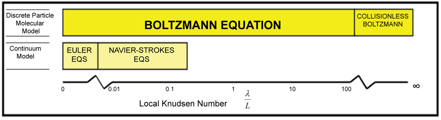


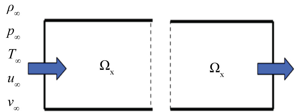
Figure 5: Inflow boundary condition...
Inflow boundary condition (left). Outflow boundary condition (right) [30].
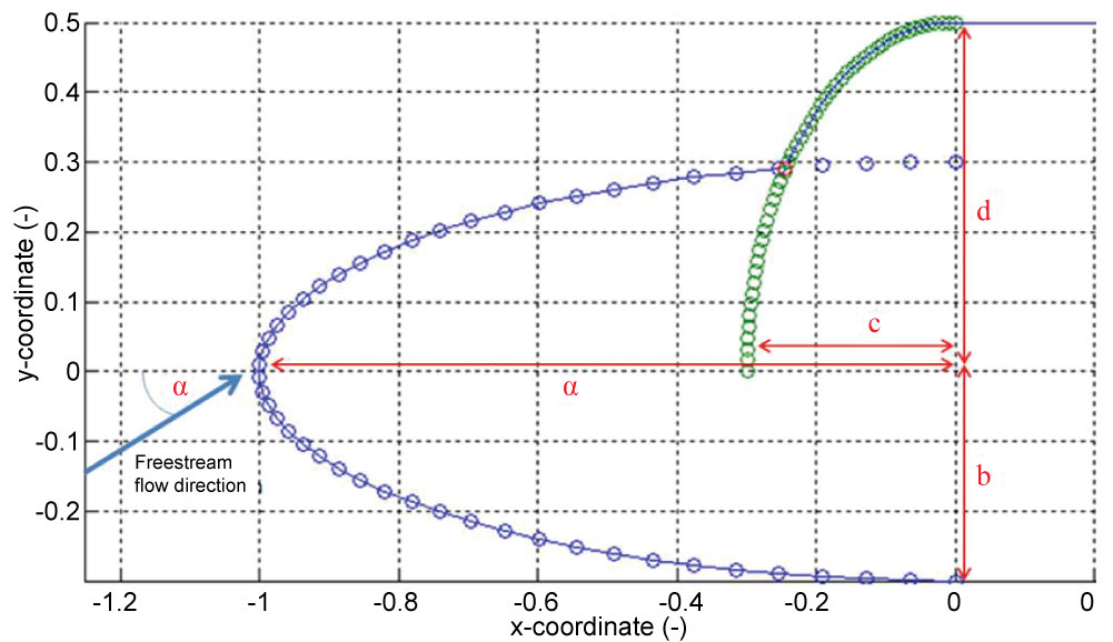
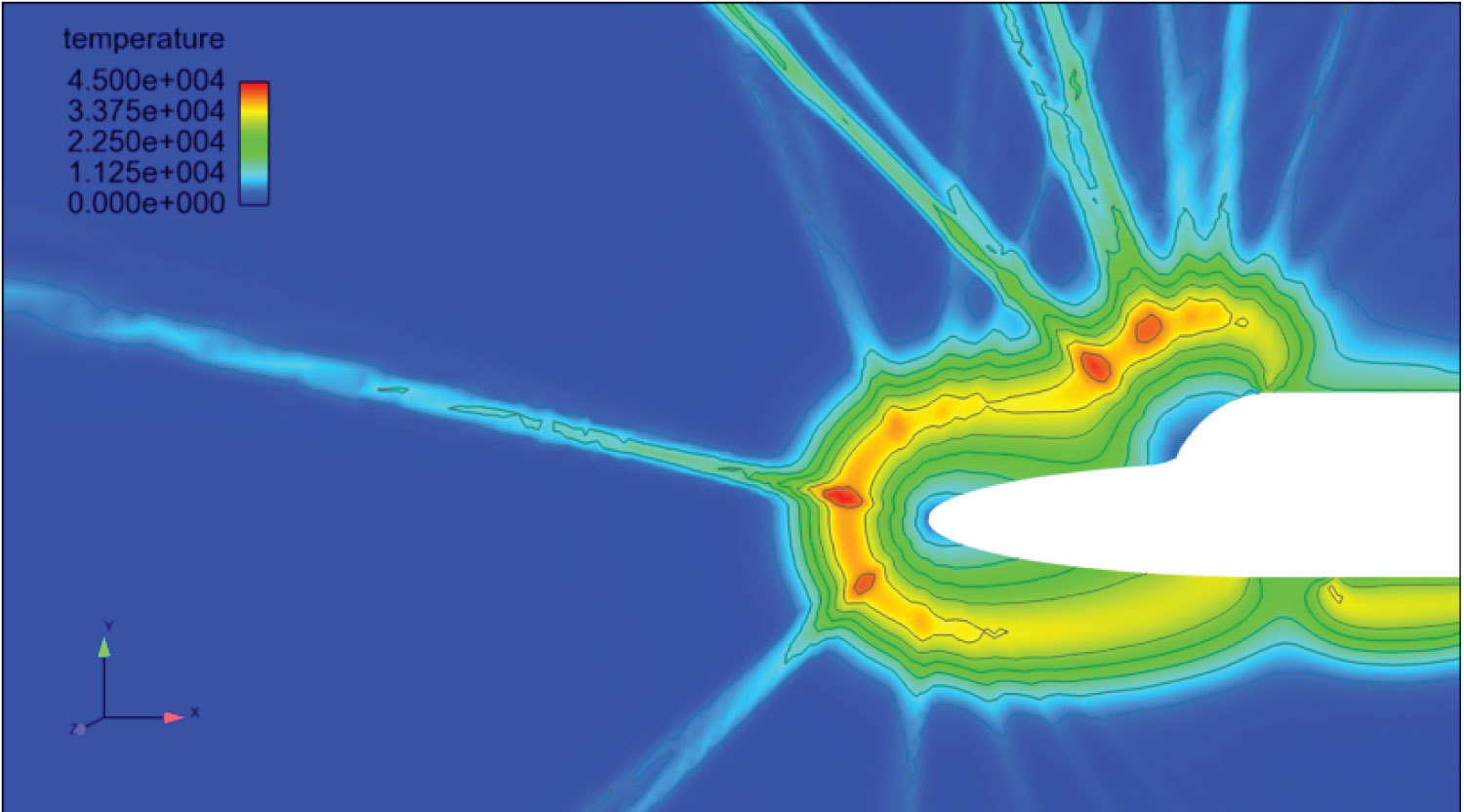
Figure 7: 80 × 80 V-Space mesh temperature...
80 × 80 V-Space mesh temperature distribution, Mach number of 25, angle of attack of 0, radial extent of V-Space of 13000 (m/s), Number of timesteps equal to 3000. Legend adjusted to show temperatures close to 45,000 Kelvin in red, 0 Kelvin in dark blue.
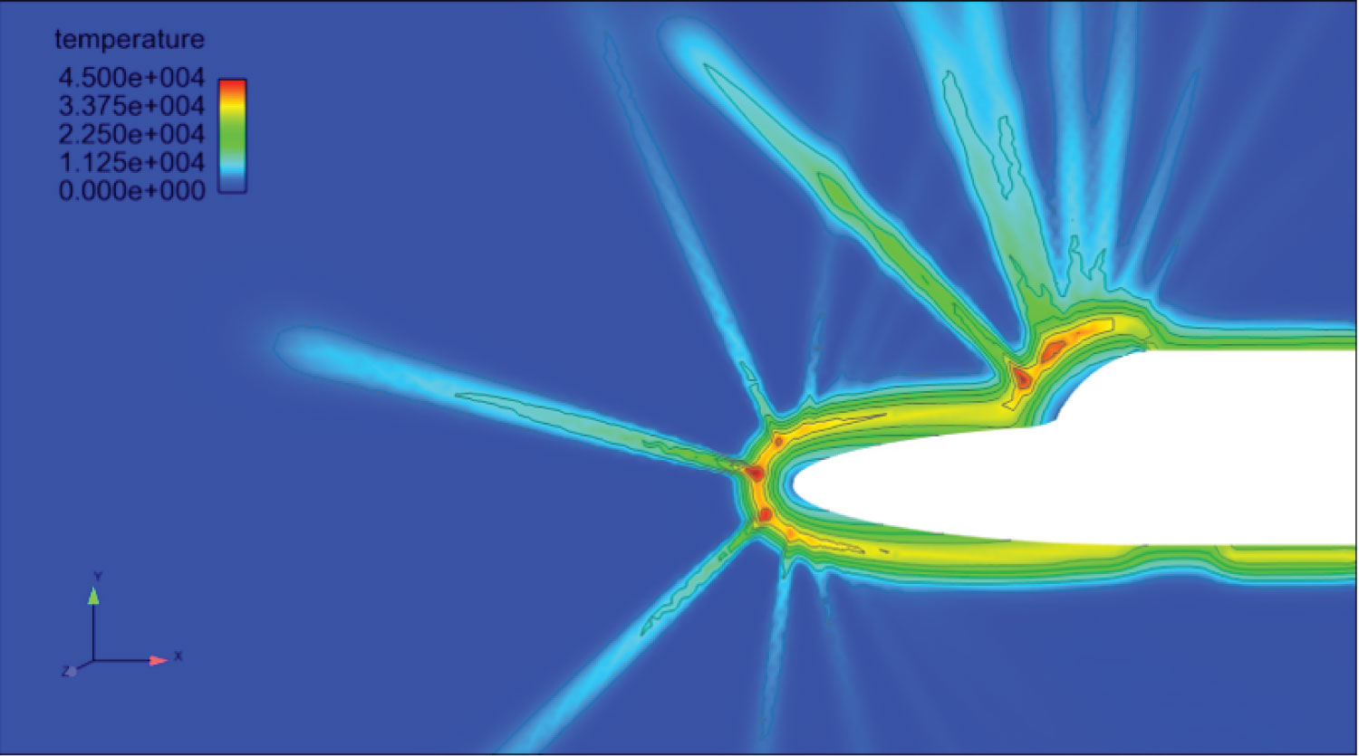
Figure 8: 120 × 120 V-Space mesh temperature...
120 × 120 V-Space mesh temperature distribution, Mach number of 25, angle of attack of 0, radial extent of V-Space of 13000 (m/s), Number of timesteps equal to 2000. Legend adjusted to show temperatures close to 45,000 Kelvin in red, 0 Kelvin in dark blue.

Figure 9: Drag comparing geometry...
Drag comparing geometry 1 (see Table 1) with Varying V-Space Mesh Distributions. Note, Drag (m2) = Drag (N) ÷ dynamic pressure (N/m2).
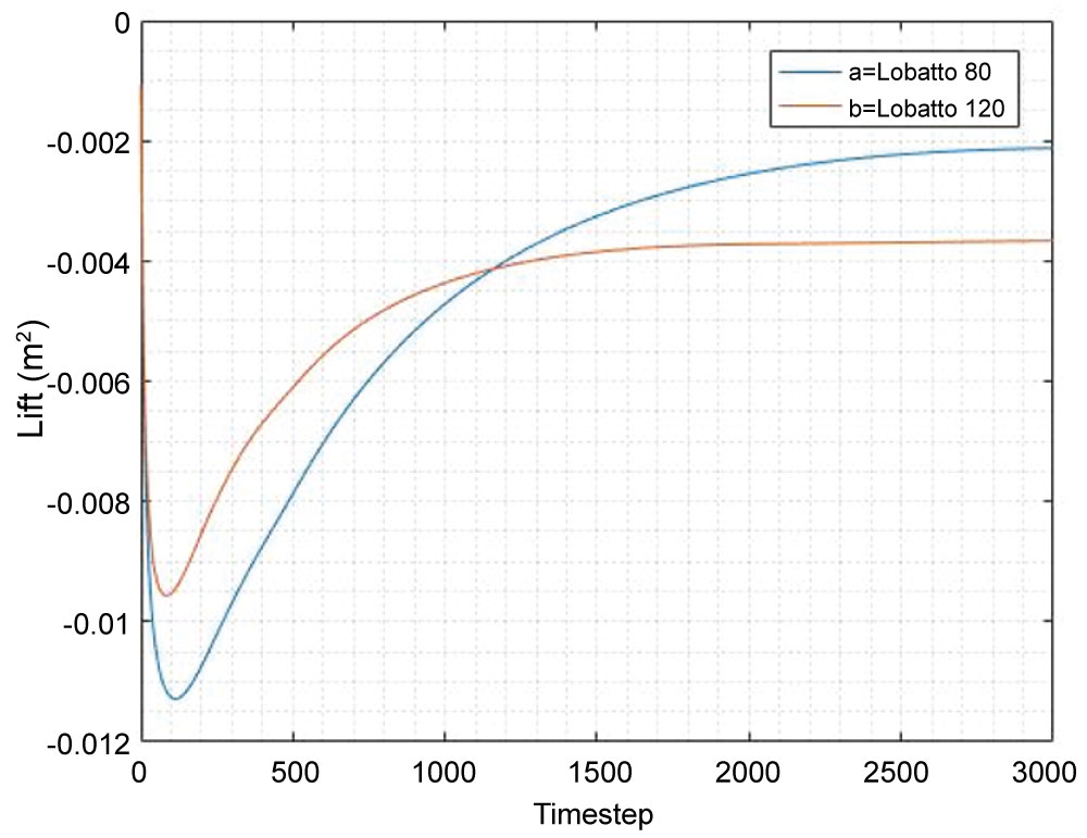
Figure 10: Lift comparing geometry 1...
Lift comparing geometry 1 (see Table 1) with varying V-Space mesh distributions. Note, Lift (m2) = Lift (N) ÷ dynamic pressure (N/m2).
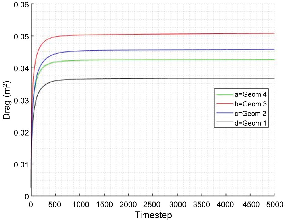
Figure 11: Drag comparing all geometries ...
Drag comparing all geometries in Table 1 under conditions of: Mach Number of 25, angle of attack of 0, radial extent of V-Space of 13000 (m/s), number of timesteps equal to 5000. Note, Drag (m2) = Drag (N) ÷ dynamic pressure (N/m2).

Figure 12: Lift comparing all geometries...
Lift comparing all geometries in Table 1 under conditions of: Mach Number of 25, angle of attack of 0, radial extent of V-Space of 13000 (m/s), number of timesteps equal to 5000. Note, Lift (m2) = Lift (N) ÷ dynamic pressure (N/m2).
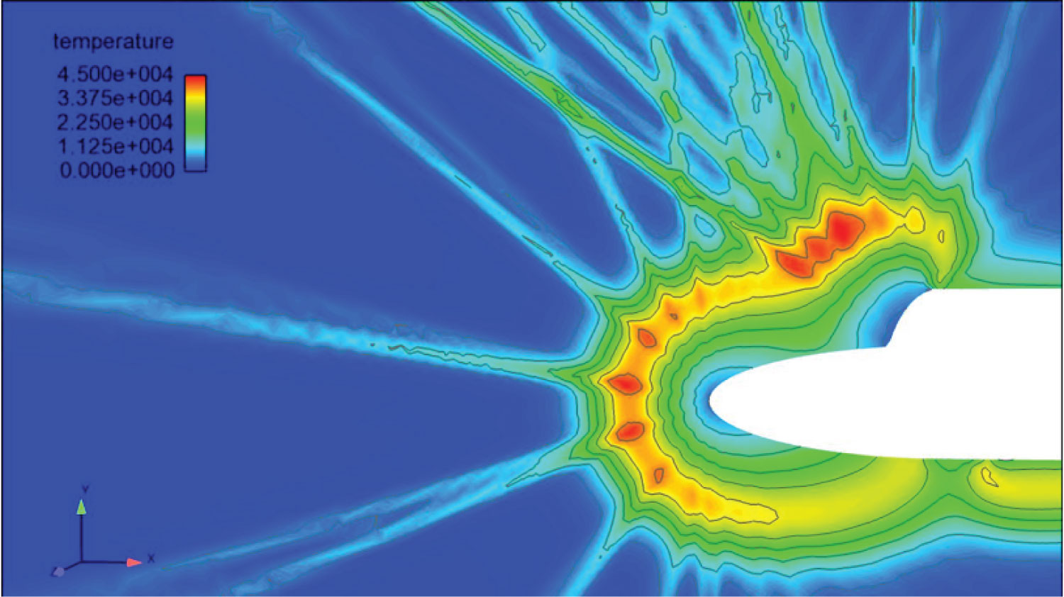
Figure 13: Geometry 2 temperature distribution...
Geometry 2 temperature distribution. Legend adjusted to show temperatures close to 45,000 Kelvin in red, 0 Kelvin in dark blue. Conditions of: Mach Number of 25, angle of attack of 0, radial extent of V-Space of 13000 (m/s), number of timesteps equal to 5000.

Figure 14: Geometry 3 temperature distribution...
Geometry 3 temperature distribution. Legend adjusted to show temperatures close to 45,000 Kelvin in red, 0 Kelvin in dark blue. Conditions of: Mach Number of 25, angle of attack of 0, radial extent of V-Space of 13000 (m/s), number of timesteps equal to 5000.
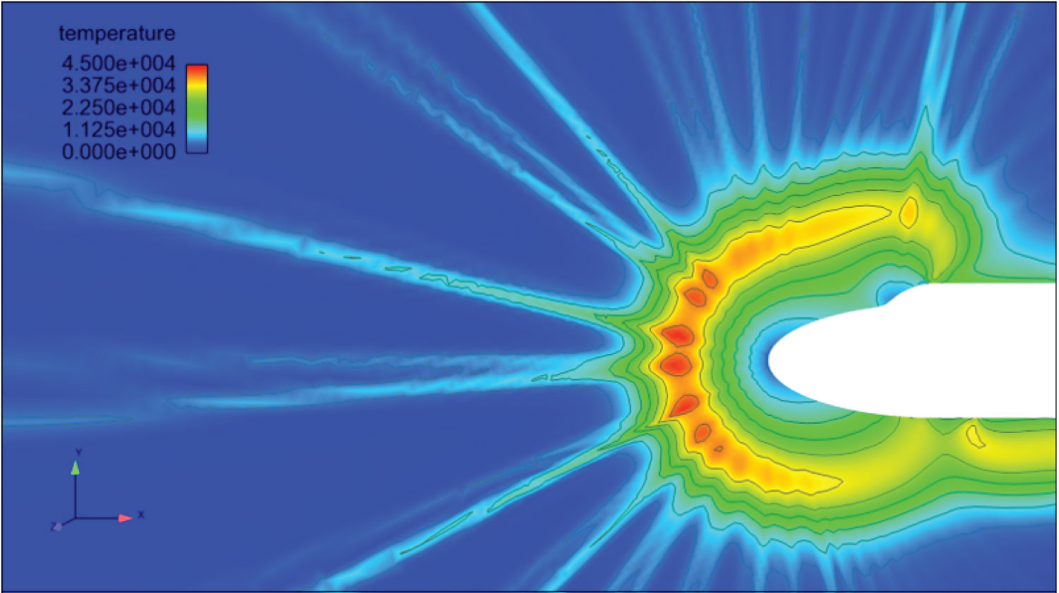
Figure 15: Geometry 4 temperature distribution...
Geometry 4 temperature distribution. Legend adjusted to show temperatures close to 45,000 Kelvin in red, 0 Kelvin in dark blue. Conditions of: Mach Number of 25, angle of attack of 0, radial extent of V-Space of 13000 (m/s), number of timesteps equal to 5000.
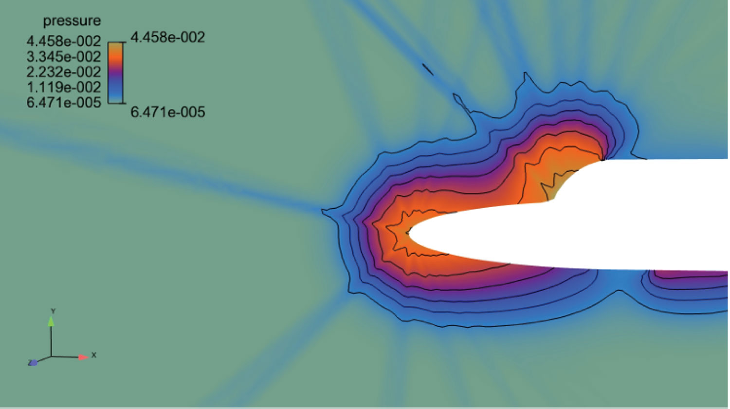
Figure 16: Geometry 1 pressure distribution...
Geometry 1 pressure distribution. Legend shows maximum and minimum values of pressure (Pascals). Conditions of: Mach Number of 25, angle of attack of 0, Radial extent of V-Space of 13000 (m/s), number of timesteps equal to 5000.
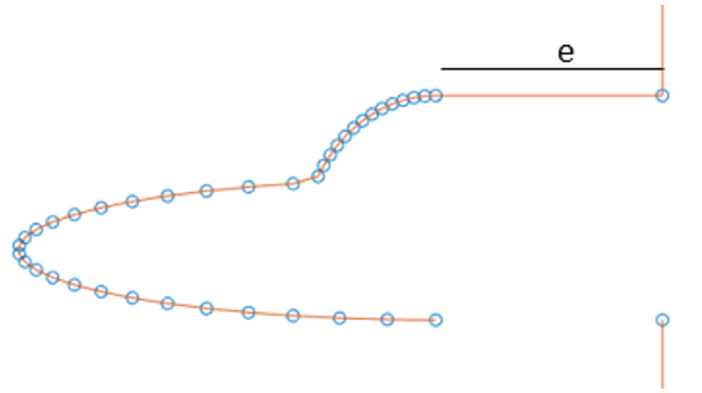
Figure 17: Body extension diagram showing...
Body extension diagram showing value of e (value of 1 in previous simulations, now 6).
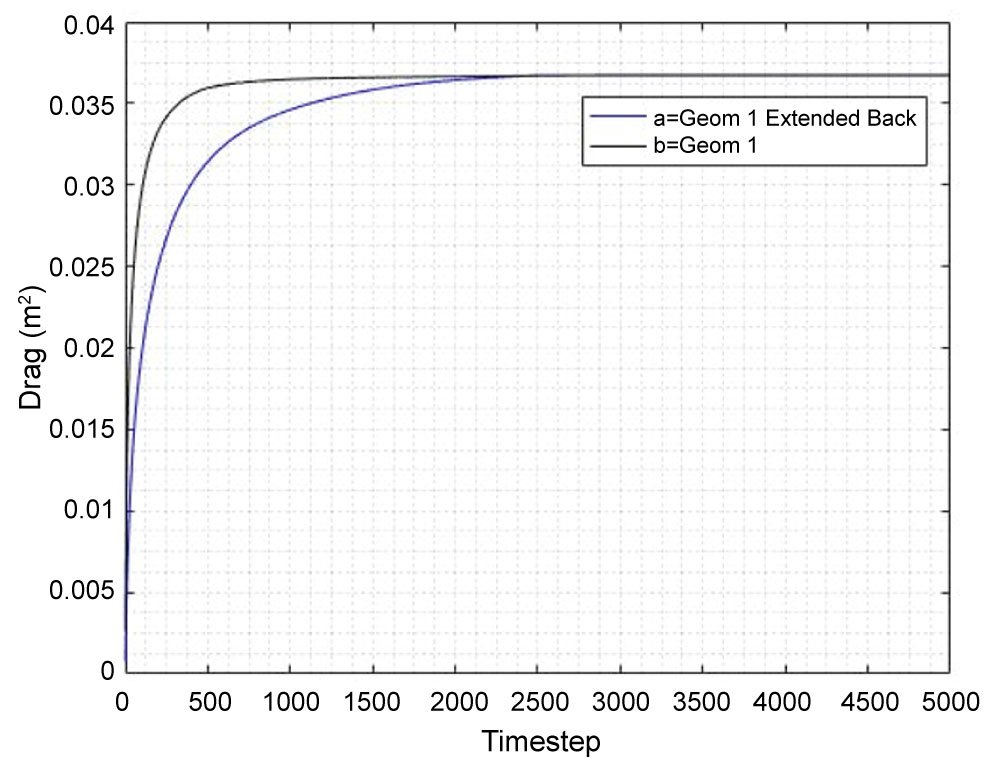
Figure 18: Drag comparing geometry 1 with...
Drag comparing geometry 1 with back extension of 1 to geometry 1 with back extension of 6. Under Conditions of: Mach Number of 25, angle of attack of 0, radial extent of V-Space of 13000 (m/s), number of timesteps equal to 5000. Note, Drag (m2) = Drag (N) ÷ Dynamic Pressure (N/m2).

Figure 19: The left side is the boundary...
The left side is the boundary condition used for all other simulations. The right side is the boundary condition for the final simulations.
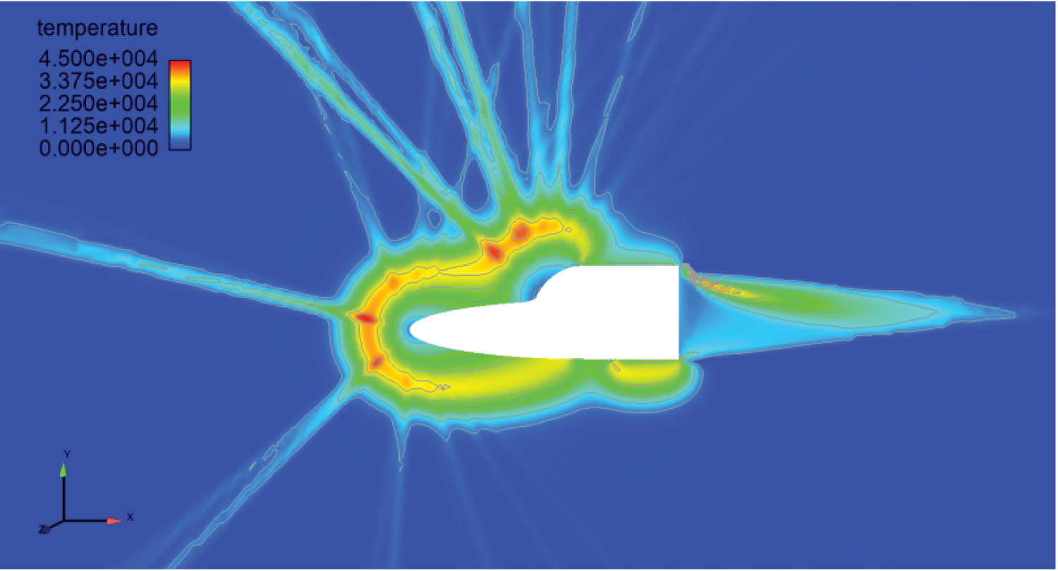
Figure 20: Geometry 1 boundary extension...
Geometry 1 boundary extension. Legend adjusted to show temperatures close to 45,000 Kelvin in red, 0 Kelvin in dark blue. Conditions of: Mach Number of 25, angle of attack of 0, radial extent of V-Space of 13000 (m/s), number of timesteps equal to 5000.
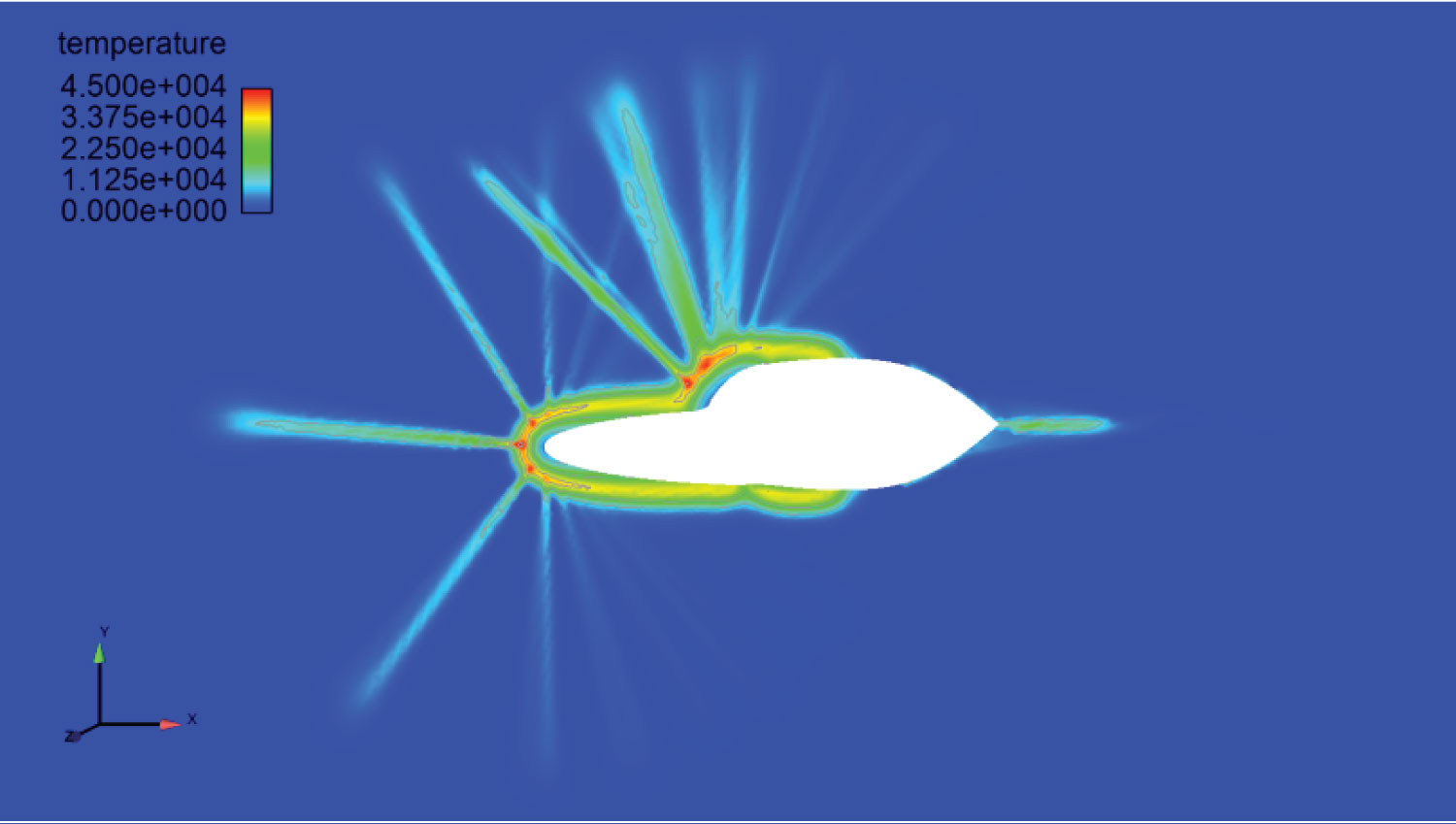
Figure 21: Geometry 1 boundary extension with...
Geometry 1 boundary extension with rounded rear. Legend adjusted to show temperatures close to 45,000 Kelvin in red, 0 Kelvin in dark blue. Conditions of: Mach number of 25, angle of attack of 0, radial extent of V-Space of 13000 (m/s), number of timesteps equal to 5000.
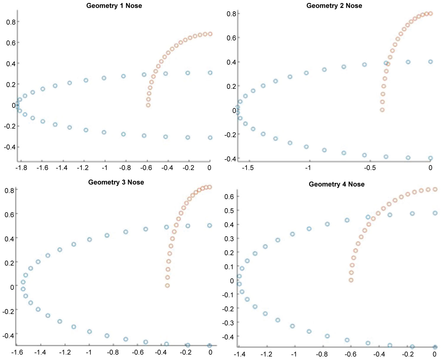
Figure 22: All nose geometries from Table 1...
All nose geometries from Table 1. Geometry 1 in top left. Geometry 2 in top right, Geometry 3 in bottom left, Geometry 4 in bottom right.
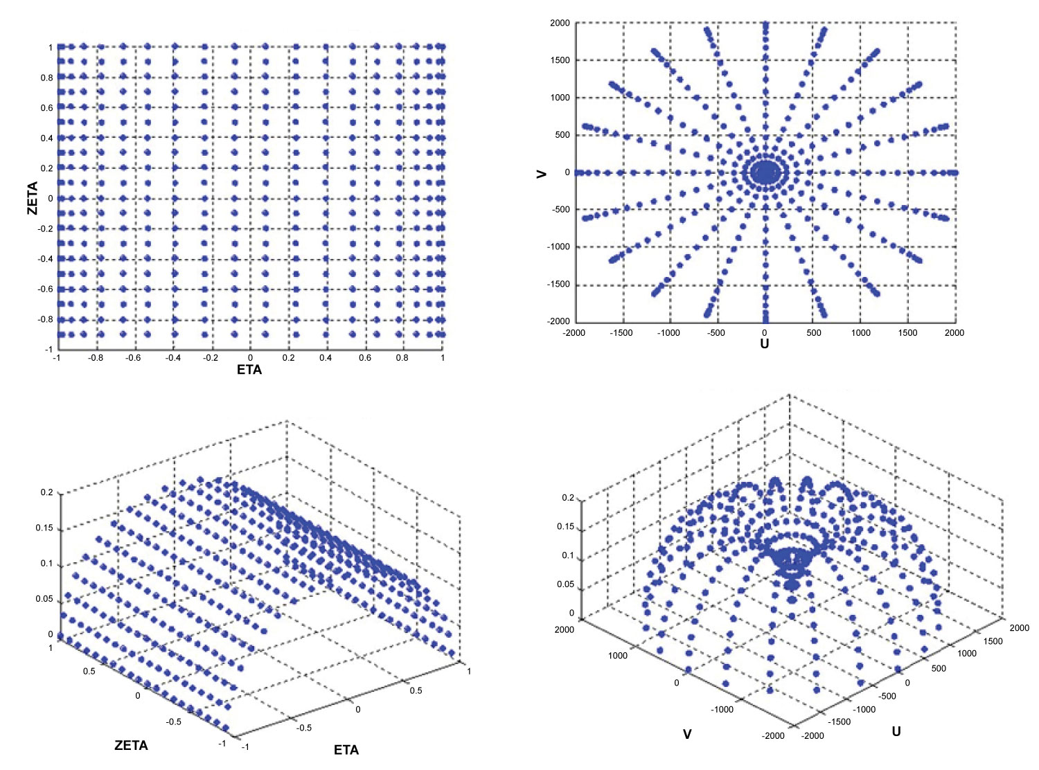
Figure 23: Velocity space discretisation diagram...
Velocity space discretisation diagram. Top Left - Coordinates of sampling points in ETA-ZETA plane spherically symmetric in real space. Top Right - Coordinates of sampling points in U-V plane, spherically symmetric. Bottom Left - Weightings in ETA-ZETA plane, spherically symmetric in real space. Bottom right - weightings in U-V Plane, spherically symmetric [10].
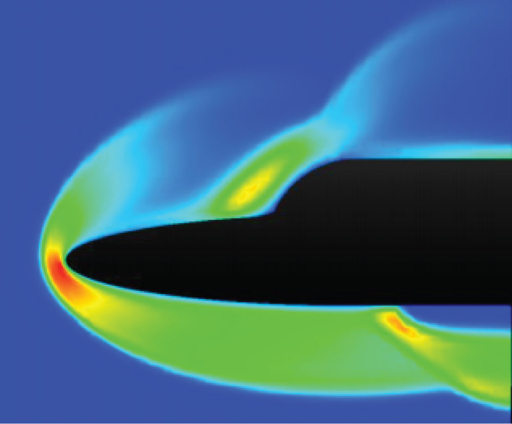
Figure 24: Low hypersonic speed simulation...
Low hypersonic speed simulation (Mach 6.5) with no numerical anomaly spikes.
Tables
Table 1: Geometric Constraints.
Table 2: Simulation Variables (unless otherwise stated).
Table 3: Rank of each geometry tested.
References
- (2017) SpaceX.
- (2017) Blue Origin.
- (2017) National Aeronautics and Space Administration.
- Topchiyan M, Kharitonov A (1994) Wind tunnels for hypersonic research (progress, problems, prospects). Journal of Applied Mechanics and Technical Physics 35: 383-395.
- (1959) North atlantic treaty organization advisory group for aeronautical research and development. design and operation of a continuous flow hypersonic wind tunnel using a two-dimensional nozzle. AGARD.
- Temam R, Lions J, Papanicolaou G, Rockafellar R (2016) Navier-Stokes Equations. Saint Louis: Elsevier Science.
- Anderson J (2010) Fundamentals of aerodynamics.
- Christodoulou D (2007) The Euler equations of compressible fluid flow. Bulletin of the American Mathematical Society 44: 581-602.
- Evans B, Morgan K, Hassan O (2011) A discontinuous finite element solution of the Boltzmann kinetic equation in collisionless and BGK forms for macroscopic gas flows. Applied Mathematical Modelling 35: 996-1015.
- Evans B, Walton S (2017) Aerodynamic optimisation of a hypersonic reentry vehicle based on solution of the Boltzmann BGK equation and evolutionary optimisation. Applied Mathematical Modelling 52: 215-240.
- Pieraccini S, Puppo G (2007) Implicit-explicit schemes for BGK kinetic equations. Journal of Scientific Computing 32: 1-28.
- Yang S, Ping C (2011) A hybrid BGK scheme for rarefied gas flow computations. AIP Conference Proceedings.
- Su W, Tang Z, He B, Cai G (2017) Stable Runge-Kutta discontinuous Galerkin solver for hypersonic rarefied gaseous flow based on 2D Boltzmann kinetic model equations. Applied Mathematics and Mechanics 38: 343-362.
- Huang J, Hsieh T, Yang J (2015) A conservative discrete ordinate method for solving semiclassical Boltzmann-BGK equation with Maxwell type wall boundary condition. Journal of Computational Physics. 290: 112-131.
- Qiu R, You Y, Zhu C, Chen R (2017) Lattice Boltzmann simulation for highspeed compressible viscous flows with a boundary layer. Applied Mathematical Modelling 48: 567-583.
- Xu K, Mao M, Tang L (2005) A multidimensional gas-kinetic BGK scheme for hypersonic viscous flow. Journal of Computational Physics 203: 405-421.
- Li Z, Peng A, Zhang H, Yang J (2015) Rarefied gas flow simulations using high-order gas-kinetic unified algorithms for Boltzmann model equations. Progress in Aerospace Sciences 74: 81-113.
- Maus J, Griffith B, Szema K, Best J (1984) Hypersonic Mach number and real gas effects on Space Shuttle Orbiteraerodynamics. Journal of Spacecraft and Rockets 21: 136-141.
- Horvath TJ, Tomek DM, Berger KT, Splinter SC, Zalameda JN, et al. (2010) The HYTHIRM project: Flight thermography of the space shuttle during hypersonic re-entry. 48th AIAA Aerospace Sciences Meeting Including the New Horizons Forum and Aerospace Exposition 2010, Article number 2010-0241.
- Bird G (2003) Molecular gas dynamics and the direct simulation of gas flows. Oxford: Clarendon Press.
- Youssefi M, Knight D (2017) Assessment of CFD capability for hypersonic shock wave laminar boundary layer interactions. Aerospace 4: 25.
- Henne P (2000) Applied computational aerodynamics. Reston: American Institute of Aeronautics and Astronautics.
- Shizgal B (1994) Rarefied gas dynamics: Space science and engineering. Washington: American Inst. of Aeronautics and Astronautics.
- Abzug M (2000) Computational flight dynamics. Reston: American Institute of Aeronautics and Astronautics.
- Cercignani C, Kremer G (2002) The Relativistic Boltzmann Equation: Theory and Applications. Basel: Birkhäuser Basel.
- Sharipov F (2015) Rarefied gas dynamics: Fundamentals for research and practice. John Wiley & Sons.
- Jain S (2007) Hypersonic Nonequilibrium Flow Simulation over a Blunt Body using BGK Method [MSc]. Texas A&M.
- Griffiths D, Margetts L, Smith I (2013) Programming the finite element method. Hoboken, NJ Wiley.
- Liu G, Quek S, The finite element method. Elsevier Science.
- Evans B (2008) Finite element solution of the Boltzmann equation for rarefied macroscopic gas flows.
- Aliabadi M, Wen P (2011) Boundary element methods in engineering and sciences. London: Imperial College Press.
- Brebbia C (1984) Boundary element techniques in computer-aided engineering. Dordrecht: Springer Netherlands.
- Hahn B (1998) Fortran 90 for scientists and engineers. London.
- Shotts EW (2012) The Linux command line. No Starch Press San Francisco, USA.
- PC Wales (2017) Swansea.ac.uk.
- Higham D, Higham N (2017) MATLAB guide. Philadelphia.
Author Details
Thomas Chiles1* and Benjamin Evans2
1Department of Engineering Science, University of Oxford, UK
2College of Engineering, Swansea University, UK
Corresponding author
Thomas Chiles, Department of Engineering Science, University of Oxford, UK.
Accepted: January 30, 2019 | Published Online: February 01, 2019
Citation: Chiles T, Evans B (2019) Computational Aerodynamic Optimisation of a 2D Space-Shuttle Geometry. Int J Astronaut Aeronautical Eng 4:022.
Copyright: © 2019 Chiles T, et al. This is an open-access article distributed under the terms of the Creative Commons Attribution License, which permits unrestricted use, distribution, and reproduction in any medium, provided the original author and source are credited.
Abstract
The need for cost minimisation in astronautical engineering, to help make human kind an interplanetary species, is not just limited to the flight and manufacturing of spacecraft. Hypersonic aerodynamic optimisation has been an expensive and time-consuming necessity since the beginning of the Apollo missions.
A Boltzmann-BGK solver developed at Swansea University is utilised in this research. Firstly, a study was undertaken to determine how the results of an arbitrary simulation would vary depending on the number of nodes in the velocity space mesh, with the higher nodal number producing a more realistic temperature distribution. The best nodal configuration found was then used to find the best nose geometry for a space shuttle during hypersonic re-entry and ascent.
An extension on the geometric variables (an increase in the space-shuttle length) was then simulated to evaluate how this changed drag results compared to an identical nose geometry with a shorter length; the results were found to be identical. Additionally, a study was undertaken to evaluate the effect of extending the outer boundary of the simulation from a half boundary to a full boundary encompassing the entire geometry, focusing on the temperature results, with a focus on the rear of the space shuttle. The full boundary extension was found to only change the temperature distribution at the rear of the geometry, the front portion of the geometry had an identical temperature distribution to the previous half-boundary simulation. Finally, the rear of the fully extended boundary simulation was altered to have a rounded rear, this was found to reduce the temperature distribution protruding from the rear.
Keywords
Boltzmann, Hypersonic, Non-continuum, Finite element, Aerodynamic optimization, Rarefied gas, Space-shuttle geometry
Introduction
The interest and need of hypersonic flight is ever expanding, both in industry and academia. As aerospace companies ranging from SpaceX [1], Blue Origin [2] to NASA [3] have clearly realised for some years now, hypersonic flight, particularly in the upper atmosphere, involves a great deal of aerodynamic optimisation, principally in the nose portion of the aircraft. Due to the reliance on wind tunnels in the sector, there are many difficulties in the hypersonic aerodynamic optimisation process. The necessity to create models to test and then recreate and retest can be very time consuming and expensive, the structural damage caused by overheating is a constant risk and the limited availability of hypersonic wind tunnels means smaller companies will have little chance to test [4,5]. There is a clear opportunity for the development of computational fluid dynamics to remove virtually all the negatives of hypersonic aerodynamic optimisation.
Computational aerodynamic optimisation practitioners have already developed effective programming software based on either Navier-Stokes [6,7] or Euler equations [8]. Due to the molecular variables of a high speed and altitude fluid differing from continuum molecular variables, the use of a more fundamental physical description must be adopted. The Boltzmann equation has been utilised in several research studies [9-17], all highlighting the potential of a novel Boltzmann solver due to its accurate use in both rarefied atmospheric conditions at hypersonic speed and more typical, low-speed atmospheric conditions. However, to the authors knowledge, no other Boltzmann-BGK based hypersonic CFD solver has been utilised for space shuttle geometry optimisation except that of Evans, et al. [9,10].
More complete studies on space shuttle aerodynamics during hypersonic flight have been completed successfully in multiple research papers. Studies such as [18] and a similar, more recent study [19], both compare hypersonic CFD data to flight data, whilst these studies are specified for comparison, they do not utilise the Boltzmann equation, hence the novelty of this paper.
Using the Finite Element Boltzmann-BGK solver developed by Evans, et al. [9], an optimised 2D space shuttle geometry will be found by simulating many different space shuttle geometries, all a 2D 'double ellipse'™ shape. A geometry which minimises drag the most on ascent will be deduced, as will a geometry that minimises temperature on descent. A compromise in the geometry will be found to find the most efficient overall geometry. The program utilises the discontinuous Taylor-Galerkin finite element method of discretisation combined with a novel optimisation approach.
Continuum equation issues
The degree to which a gas can be considered rarefied can be expressed through the value of its Knudsen number, Kn, This is a non-dimensional quantity defined as
Where L is any characteristic dimension in the flow and λ is the mean free path of the molecules, i.e. the average distance travelled between collisions.
The typical assumption that the Navier-Stokes equations are no longer valid if the Knudsen number is greater than 0.1 [20] is misleading if any overall dimension of the flow L has been chosen. The limit of the continuum equations should therefore be specified using a local Knudsen number where L is defined as
Where L is now the scale length of the macroscopic gradients [20] and ρ is the density of the fluid. A diagram showing the appropriateness of a range of equations at various Knudsen number can be found in Figure 1.
A diagram showing the appropriateness of a range of equations at various Knudsen number can be found in Figure 1.
Viewing Figure 1, it is clear to the reader that a computation utilising the continuum model will not be appropriate for a solver in rarefied atmospheric conditions. Continuum theory always assumes that a gas is in thermodynamic equilibrium, i.e. in thermal, chemical and mechanical equilibrium, however in this paper, the gas analysed will not have the appropriate time needed to return to equilibrium and so a separate set of equations must be utilised. The inaccuracies of using non-equilibrium Navier-Stokes equations can be found in [21].
For examples of other techniques and equations utilised in computational aerodynamics, see [22-24].
Boltzmann equation
A detailed description of the Boltzmann equation theory and application can be found in [25,26]. The reader is again directed to Figure 1, where the accuracy of using a Boltzmann type solver is highlighted graphically. The Boltzmann equation accurately describes a fluid that is not in a state of equilibrium [23].
Maxwell distribution function
At this time, it is appropriate to introduce the Maxwellian distribution function to the reader. This function will be used in the Boltzmann-BGK solver as it allows the equation to still be a non-linear integro-differential equation [9] whilst applying the BGK approximation to simplify the computation.
The Maxwellian distribution form applied to the Boltzmann-BGK solver is
Where c0 is the bulk velocity of the flow, c is the velocity of the flow and . T equals the temperature of gas (measured in Kelvin), m is the molecular mass, R is the molar gas constant and k is the Boltzmann constant [9]. Further detail about this function can be found in [9,26].
Equation (3) is the three dimensional form of the equation, the two dimensional form of the equation is
Where the only difference between equations (3) and (4) are the β and π powers.
Boltzmann-BGK equation
The simplification made by Bhatnager, Gross and Krook (BGK) in the Boltzmann equation assumes that the departures of the flow from thermodynamic equilibrium are small. A further assumption deduced from their conclusion is that the effect of the molecular collisions in a non-equilibrium fluid, forces the non-equilibrium molecular velocity distribution back toward a state of equilibrium, at a rate proportional to the molecular collision frequency [10]. The Boltzmann-BGK equation may be written as
Where n is the molecular number density, F takes into account any force fields that are present, f = f(r,c,t) is the molecular distribution function of the fluid, 𝒱(r,t) is a mathematical term proportional to the collision frequency of the molecules, r represents the position of the molecules and f0 is the local Maxwellian equilibrium distribution function discussed above.
A direct comparison between a Boltzmann-BGK scheme and a continuum scheme can be found in [27] where the Boltzmann-BGK solver is found to be more accurate at modelling shock tube problems.
Boltzmann-BGK Solver
The reader will now be given a brief explanation of some of the key aspects of the Boltzmann-BGK solver developed by Evans, for a more detailed explanation, see [9,10].
Physical space discretisation
The Boltzmann-BGK solver is restricted to two physical space dimension problems. The physical space is referred to as p-space domain, Ωr. The p-space domain is discretised into a linear, discontinuous, triangle element, unstructured mesh (Figure 2). There are multiple advantages to using a discretisation technique of this nature [9,10] but it is specifically utilised for rarefied hypersonic flow because of the shock capturing properties. For further discretisation techniques, the reader is directed to [28,29].
Velocity space discretisation
The velocity space is referred to as the v-space domain, Ωc, and theoretically is unlimited in extent, however to create a working solution to the solver, a limit on the maximum velocity of molecules is identified; any molecule travelling faster than this is assumed to have negligible impact on the solver accuracy. To apply this principle to the Boltzmann-BGK solution, an estimate of the mean thermal molecular velocity must be made by using moment calculations (see [9,10] for full mathematical description). The relationship between the thermal molecular velocity and other flow variables is found to be
Where is the mean thermal molecular velocity. The finite limit of the radial extent of the velocity domain, rv, can be viewed in Figure 3.
A spectral v-space domain is a single, high order element [9] and so gives for more efficient calculations over the full domain. To apply this domain, it must first be mapped from Cartesian or polar coordinates (in real space), to a quadrilateral element in the (η, ζ) plane.
View Figure 4 to see the mapping of the quadrilateral element. The mathematics of this approach can be found in [9,10] but a detailed understanding of this method is not necessary to the reader. This method creates a symmetric distribution of points, with no preference on a radial direction.
Taylor-Galerkin discretisation method
A summarised explanation of the Taylor-Galerkin discretisation will now be highlighted, for a more in-depth description, see [9,10,30].
An approximation is used in this method
Where f is the distribution function, n is the molecular number density, implies the value of nf at timestep of m + 1/2 and spatial coordinates i.e Q = v(r,t)((nf0 )- (nf)) where f0 is equation (4).
Step 1)
The piecewise-constant increment is calculated at every physical space element, using the equation
Where Δ(nf)re,c is the piecewise-constant increment, Δt is the timestep (global), k is the summation that extends over three nodes of the element re, Nk is the finite element shape function at node k (piecewise-linear) and
Element fluxes during a timestep of a half are calculated using the piecewise linear discontinuous equation
Step 2
The last step involves a piecewise-linear approximation for Δ(nf) at every physical space element. All element node values of the solution increment over the complete timestep [10] are calculated using the equation
Where is the normal component of the upstream flux at the physical space element edges, ML]re is the 3 × 3, physical space element mass matrix, Ωre,c is the physical space element domain, Γre is the physical space element boundary.
Boundary conditions
Three key boundary conditions have been applied to the Boltzmann-BGK solver: Inflow, outflow and wall. An explanation of each boundary condition and their relevant equations can be found in [9,10,30]. These boundary conditions are applied accurately to the solver by modelling of , a part of equation (11). A brief explanation of each boundary condition will now be given.
Inflow
All gas properties necessary to calculate the Maxwellian distribution function in two dimensions, see equation (4), are present. It is now possible to calculate the inter-element flux at the inflow using equation
For molecular velocity directed into the domain. For molecular velocity directed out of the domain, equation (9) is utilised.
See Figure 5 for a visual representation of the inflow boundary condition, where all of the gas properties needed for calculations are represented.
Outflow
The inter-element calculations at the outflow boundary domain is more simplistic then at the inflow, as it is not dependant on the direction of molecular velocity.
The inter-element flux equation is
Figure 5 shows a visual representation of the outflow boundary condition.
Wall
The wall condition means that the value for mass flux across the boundary is zero [9,10,30]. This is represented in the equation
Where Γr is the physical space domain boundary [9,10,30] and Fn,c = (c.n) f(c,r,t).
For further boundary conditions examples, see [31,32].
Parallelisation
For the Boltzmann-BGK solver to be applied to complex problems and work in a reasonable timeframe, the use of parallelisation in the code is necessary. The method chosen is physical space domain decomposition.
The information communicated between each processor is that of the inter-element flux. It is noted that the flux information can only be communicated in one direction and never both directions at the same time, for example, processor 1 will pass its inter-element flux information to processor 2 (left to right) but then processor 2 can only pass on its inter-element flux information to processor 3 (left to right, not right to left). The direction that the information travels is dependent on the molecular velocity vector.
For a more complete description of the parallelisation process used, see [30].
Software and Hardware
The solver developed by Evans is coded in the FORTRAN 90 language, this language was chosen due to the allocable memory and speed of computation [33]. In this authors research, the solver was compiled and run using a Unix cluster account [34] and utilised the power of the Swansea University High Performance Computing (HPC) facility [35]. The alterations to the space-shuttle geometry were all completed using Matlab software due to its simplicity at plotting two dimensional shapes [36].
Generating Geometry
Figure 6 shows a diagram of the space shuttle geometry variables that were altered. Values of a, b, c and d were changed during each new geometry simulation.
Table 1 shows the geometries that have been produced and were simulated. Note, a visual representation of each geometry can be found in the Appendix.
V-Space Node Value Study
A study was undertaken to determine how the results of an arbitrary simulation will vary depending on the number of nodes in the v-space mesh. Note that the geometry in this study is geometry 1 in Table 1. See Appendix for a diagram of points in the velocity space discretisation.
Lobatto 80 Quadrature
This v-space mesh contained a number of nodes equal to 80 × 80, i.e. 6400 nodes. Figure 7 shows the temperature distribution for the Lobatto 80 simulation.
Lobatto 120 Quadrature
The v-space mesh was then changed to contain a 120 × 120 mesh, i.e. 14400 nodes in total. Figure 8 shows the temperature distribution for the Lobatto 120 simulation.
Results
The lower v-space mesh simulation needed 1000 more timesteps than the higher v-space mesh simulation to gain results with low variation of lift and drag (view Figure 9 for the drag variation and Figure 10 for the lift distribution). However, it is clear from these figures that the variations in both drag and lift results are small (less than 0.01 difference) and so the necessary increase in time needed to use a Lobatto 120 × 120 v-space mesh in a simulation may not be ideal when considering the relative accuracy of the Lobatto 80 × 80 results (which takes far less time to run, around 24 hours less).
Comparing Figure 7 and Figure 8, it is clear that the temperature variations have similar values (the reader is directed to the bottom-right corner of both figures). The Lobatto 120 × 120 simulation has a more condensed temperature distribution then the Lobatto 80 × 80 simulation, this is due to the higher density of v-space meshing which has produced a more realistic temperature distribution.
Introduction to Simulation
Simulation variables
Table 2 shows the variables chosen for all simulations in this research. These values were chosen as these conditions are roughly the most extreme conditions a space shuttle will experience during its product life.
Data
Data is used to evaluate two things: the drag that the simulation produces, and whether the simulation has converged to produce accurate results (produces a flat line, see Figure 9 and Figure 10 for examples of this).
The data for geometries 1 to 4 are presented in Figure 11 and Figure 12. These simulations have been produced using the conditions stated in Table 2.
Figure 11 and Figure 12 show that all geometries produce results for lift (Figure 12) and drag (Figure 11) to steady state (minimum 3 significant figures), this is why all lines are flat by 5000 timesteps. This suggests that all results are reliable.
Simulation 1 - Hypersonic Re-entry
Aims of hypersonic re-entry simulation
This simulation was utilised to evaluate the 4 geometries specified in Table 1. The aim of this simulation was to find the best geometry of the 4 during hypersonic re-entry.
Temperature minimisation
The temperature that the geometry experiences needs to be minimised, particularly during hypersonic re-entry due to the large values of temperature produced at this speed when reentering the Earth'™s atmosphere. The large temperature can cause structural damage and even failure in some severe cases.
Lift minimisation
Lift needs to be minimised during re-entry. More lift will make it more difficult for a spacecraft to successfully re-enter the atmosphere and come to a controlled landing.
Results
Note that Figure 7 shows the temperature distribution for geometry 1 (Table 1).
Viewing the temperatures distributions in Figure 7, Figure 13, Figure 14, and Figure 15, it is clear that Figure 7 (geometry 1 in Table 1) has the most success in minimising temperature under identical conditions. All figures have the same temperature scale (45,000 Kelvin is red, 0 Kelvin is dark blue) and Figure 7 has by far the least 45,000 Kelvin temperature regions.
Geometry 1 also is the best geometry evaluated in terms of lift minimisation. Viewing Figure 12, geometry 1 flattens out at a steady state solution for lift at a lower value than all other geometries. Note that geometry 2 is the next best geometry for lift minimisation.
Figure 16 shows the pressure distribution of the best geometry for hypersonic re-entry (geometry 1).
Note, the striations in the temperature and pressure figures are caused by a numerical anomaly produced when using high order spectral discretisation of the velocity space. This is an area of ongoing research in the field of high speed computational aerodynamics.
Simulation 2 - Ascent
Aims of ascent simulation
This simulation was again evaluating the 4 geometries specified in Table 1. The aim of this simulation was to find the best geometry of the 4 during the ascent phase of a shuttle mission.
Drag minimisation
It is necessary to minimise drag during the ascent phase of a space mission, as this will minimise the amount of thrust needed to reach space. Less drag also means a smaller net force acting upon the structure, decreasing the likeliness of failure of the structure.
Results
Figure 11 shows that geometry 1 (Table 1) is once again the best geometry. It creates the lowest value of drag, 0.036 m2. Note, geometry 4 is the second best at minimising drag.
It is clear from Table 3 that geometry 1 is the ideal geometry for use at any stage in a space-shuttles flight; therefore this geometry will now be evaluated further by expanding geometric parameters.
Simulation 3 - Increased Shuttle Geometry Parameters
Body extension
Geometry 1 variables were then used to form the front nose geometry, however, the body of the geometry was extended to evaluate its effect on drag. A visual representation of this can be seen in Figure 17.
The value of e was 6 (corresponding to Figure 18 and Figure 19). The reader should note that all previous simulations were limited to an e of 1.
The drag results for this body extension simulation are then compared to Figure 7 (same nose geometry, a back extension of 1).
Only the drag results are considered due to issues with the lift not converging in the allotted timesteps. However, the drag converges quickly to a steady state solution in 5000 timesteps and so can be compared to the geometry 1 drag results (Figure 18).
Results-body extension
Viewing Figure 18, it is clear that both standard geometry 1 and geometry 1 extended back converge to an identical drag value of 0.036 m2. Note that geometry 1 extended back converges to a steady state value less efficiently than standard geometry 1, this is expected as having a larger geometry in the simulation involves a larger number of calculations and therefore processing time.
Boundary extension
A final simulation was then completed with the boundary of the simulation extended to surround the entire geometry, so the temperature distribution can be analysed (Figure 19). The temperature results from this simulation are then compared to the original geometry 1 temperature results, whilst also being compared to an identical geometry with a rounded rear. Note, the effect the rear of the geometry (now included in the full boundary simulation) has on the temperature distribution is a particular focus.
Results-boundary extension
Figure 20 shows an identical space shuttle geometry to that of Figure 7, however Figure 20 has a rounded boundary. This boundary extension has the effect of producing a temperature distribution protruding from the rear of the geometry, creating a more realistic temperature distribution than that of the halfboundary simulation in Figure 7. This is the only difference between the full boundary and half boundary temperature distributions, both have an identical distribution when considering only the temperature effect on the front portion of the geometry.
Viewing Figure 21, this geometry has a rounded rear to its design. Comparing this to Figure 20, the rounded rear of Figure 21 causes the temperature at the rear of the geometry to significantly decrease in both magnitude and area.
The rounded rear of Figure 21 also influences the temperature distribution at the front of the geometry. Much like when comparing v-space nodal values, the distribution values are virtually identical, but Figure 21 has a more condensed distribution then that of Figure 20.
Conclusion
This research has outlined the potential of hypersonic aerodynamic analysis using a novel Boltzmann-BGK solver. Issues with the solver have been highlighted, these include: being computationally expensive to run and a numerical anomaly produced when applying high order spectral discretisation of the velocity space.
Issues aside, the power of this solver has been presented by simulating a number of scenarios that are applicable to a space shuttle mission. The success of this solver under different scenarios paves the way for further development in hypersonic Boltzmann based solvers with the hope of complete reliance on computational data for aerodynamic optimisation in the future.
The solver used must first be compared to accurate data from a source outside of computational aerodynamics before further development into a potential 3D aerodynamic package can be produced.
Once further development is completed on this unique solver, a more large scale research project, similar to [18-19] can be completed.