Accepted: January 21, 2023 | Published Online: January 23, 2023

Citation: Eben-Chaime M (2023) Time and Cost Control in Projects: An Engineering Approach. Int J Ind Operations Res 6:015.

Copyright: © 2023 Eben-Chaime M. This is an open-access article distributed under the terms of the Creative Commons Attribution License, which permits unrestricted use, distribution, and reproduction in any medium, provided the original author and source are credited.

Abstract

In this paper, an engineering approach is proposed for time and cost control in projects. It has been observed for long time and by various authors, that project cost forecasting becomes very accurate over time, whereas duration forecasting is not reliably accurate. A sound reason is the fundamental difference between project's schedule and costs. Total project's cost is the sum of all the cost components, whereas project's duration is determined not by all its activities, but only by the subset of critical activities. The inaptness of using sums for schedule/time control is demonstrated in this study. Yet, prevalent methods still use sums for schedule control. Moreover, project control is not aimed at forecasting but at projects' successful completion. In response, the 'engineering' approach is proposed, as an alternative. Under this approach, control data is analyzed at the activity level and then synthesized to the project level according to the precedence and other constraints. This facilitates the major control functions: diagnosis and selection of responses, and estimations, too. Further, the proposed approach is applicable to cost control, too, and offers means to handle the troubling level-of-effort costs.

Keywords

Project control, Earned value, Estimate at completion, Level of effort

Introduction

Project control is not only the longest task in project management (PM) but most significant, too. Even a perfect plan would not suffices for project's success if not properly executed. "The main goal of PM and project control in particular is to finish a project within budget and before a specified deadline, while fulfilling customer requirements." [1] Not all projects are conducted for customers, but: "…, most projects are initiated by a need. … When management is convinced that the need is genuine, goals may be defined." [2], (page 6). Consequently, the scope of PM is to achieve the defined goals within budget and before a specified deadline. These three dimensions: scope, time and costs, are interrelated, but this study is primarily focused on the time, or schedule, and costs.

Projects usually involve high degree of uncertainty. Thus, project plans rely on estimations, which are prone to errors. Uncertainty and project control have also been considered (e.g., [3]). Moreover, projects last time, very often long time. As in statistical estimations (e.g., [4]), the further the extrapolation the lesser is the accuracy. Predicting far into the future decreases the value of the various estimations which have been used in planning the project. Due to the combined effects of uncertainty and long duration, projects must be monitored along their execution to make sure the progress is as planned, take corrective actions when desired and/or change the expectations - this is the mission of project control. The need to monitor tasks with long durations has also been observed by Li and Zhong [5] who noticed the similarity to PM but underlined the differences, too.

Projects usually involve high degree of uncertainty. Thus, project plans rely on estimations, which are prone to errors. Uncertainty and project control have also been considered (e.g., [3]). Moreover, projects last time, very often long time. As in statistical estimations (e.g., [4]), the further the extrapolation the lesser is the accuracy. Predicting far into the future decreases the value of the various estimations which have been used in planning the project. Due to the combined effects of uncertainty and long duration, projects must be monitored along their execution to make sure the progress is as planned, take corrective actions when desired and/or change the expectations - this is the mission of project control. The need to monitor tasks with long durations has also been observed by Li and Zhong [5] who noticed the similarity to PM but underlined the differences, too.

The paper is structured as follows. The relevant literature is concisely reviewed in the next section and to better position this study, control and project control are generally, but briefly discussed in Section3. In Section 4, the need is proven by demonstrating flaws with existing approaches. A solution - engineering project control (EPC) is proposed in Section 5 and the discussion is extended to costs in Section 6. A summary and directions for future studies are offered in Section 7.

Literature Review

Several reviews of the literature on project control have been published in recent years (e.g., [1,10,11]). From these reviews, the following issues are relevant to this study: 1) Trends in the selection of methods and techniques, 2) The popularity of the earned value method (EVM) and its derivatives for projects' costs and time control, 3) The lesser accuracy of time EAC, as noted above, and 4) The emphasis on the big picture, i.e., total duration and total costs at each stage, ignoring the build-up of these figures and measures [6].

Traditional methods and techniques for project planning and control are based on deterministic network models (e.g., [10]). This includes the critical path method (CPM). The development of the CPM in the late 1950s and is one of the foremost breakthroughs in modern management as it enables the planning of projects of almost any size. However, a shift from these methods has been observed [10] and of the 187 papers surveyed in [1] only four included project networks. There is a fundamental difference between cost and time. Project's direct cost weakly dependent on the order of execution and equals the sum of the costs of all project's components. Projects' duration, on the other hand, strongly depends on precedence constraint and schedule. Consequently, project's duration is determined not by all its activities, but only by a subset of them - the critical activities. The notion of critical activities is an elementary component of traditional PM tools like the CPM (e.g., [2]) and the critical chain [12]. Users of PM software tools may be unaware of it, but since project scheduling must account for precedence constraints, most, if not all these tools employ network models. This can be observed in the screen-shots printed in (e.g., [6] and [13]), by the arrows which connect activities. Thus, the integration of these issues in project control is inevitable.

A tool which has been proven useful for cost control is the earned value method (EVM) (e.g., [14] and [15]). This method has been used since the 1960's by U.S. government agencies and following its success, an industrial standard has been issued [16]. Consequently, the EVM is very popular. Some examples of the wide range of application domains and project sizes can be found in [8,9,13,17,18]. However, EVM was originally developed as a cost management and control tool, which has been extended to track the schedule as well [11]. Consequently, it should be no wonder that the time estimations of the EVM are of lesser quality and hence used less. Few derivatives has been proposed to improve the value of the estimation of the earned portion of the work content; e.g., the earned schedule (ES) method [8] and earned duration(ED) method [6]. Studies have then been conducted to compare these methods (e.g., [13]). The approach proposed here is different and can hence be used in conjunction with any of these methods.

In addition, studies on time-cost control, and EVM in particular, "focus on the big picture cost and duration within certain stages of a project" [11]. While in [6] and [13] the values at the project level are all calculated as sums of the corresponding values of the individual activities, all other references consider only the project level. This includes both progress and estimation performance measures, the schedule compliance (c factor) and the schedule adherence (p factor) [13], in particular. As noted above and demonstrated later, due to precedence constraints, projects' duration is, usually, not the sum of the durations of all the activities, but only of some of them. Further, as projects move on, critical activities might turn non-critical and vice versa. Moreover, all the estimations are naïve (e.g., [19]) - projecting the past on the future making no attempt to understand how things evolved and how the project arrived to its current situation.

Following the discussion thus far, three principles comprise the theme of the proposed engineering approach. First, project control is not about updating the estimations, but about the accomplishment of project's goals within budget and on time. Estimations should be used for decision support. Second, projects are governed by precedence constraints, which hence, cannot be avoided throughout the lifecycle of the project, including project control. Third, for better and more effective project control, and more accurate estimations as well, performance should be analyzed at the activity level. The results should then be synthesized to the project level in accordance with the precedence and other constraints; e.g., resources.

Project Control

Upon looking in dictionaries: Cambridge, Oxford, Merriam-Webster, the closest to the word 'control' are the words govern as a verb and governance as a noun. Project control, however, amounts to more and is actually a 'control system'. Further, since projects are continually modulated, project control is a closed-loop or feedback control system. Feedback control systems are aimed and attempt to make and keep the controlled entity - object or system, behave and perform as desired (e.g., [20], chapter 4). This implies the existence of, at least an implicit perception of what is 'as desired'; e.g., project plan, and of means to compare reality to plans and make changes, when desired. Aware or unaware, explicitly or implicitly, control actions are performed continually and anywhere, including in daily activities; e.g. setting/changing the water temperature in a tap, adding spices to the food, etc.

Originally, in unmanned systems, the control system changes the functionality of the controlled entity; e.g., turning the AC 'on' or 'off' or accelerating or slowing a car. Human involvement adds another facet to the control system - expectations, which can also be changed (e.g., [21]). Car driving is an excellent example of control, including this facet. Most car trips are made for certain purposes. Often, others are expecting the passengers in the destination. If late arrival is estimated either the speed can be increased - a functional change, or the arrival time can be updated - change of expectation (or the flight is missed).

As already noticed, most projects are initiated by needs. These needs are, hence, the primary concern of project control, which should make sure that the effort is maintained directed towards responses which are worthy of the needs and will meet the expectations. Time and costs are additional concerns. The scope-time-cost triangle plays an important role in project control. Since resources involve costs, changing the rate of progress might result in cost changes; e.g., it is commonly assumed that speeding the progress usually involve higher cost, in any case, these are functional changes. Changes of project's scope are changes of expectations, which are often required to keep the project on schedule and/or within budget. Yet, it might also happen that thing go better than expected, in which case the scope can be broaden and/or time and costs be saved. Either way, it is critical to identify the gaps as soon as possible, either to mitigate or to get ready to materialize opportunities.

In sum, projects are initiated by needs. Once the needs are identified, goals are set and the response to the needs is designed. Control begins right in these initial stages with the, so called, configuration control, which is aimed, at this time, at the quality of design - to guaranty that the best response is offered to the needs. Later, configuration control is in charge of controlling design changes. Upon approval of the design, a plan is developed for the project, which is reflected in its budget. Then, the execution phase begins, which requires the majority of the control effort and during which time and costs are also controlled. Reality is then compared to the plan and in the presence of variances, diagnosis is required, decisions should be made how to tackle the deviations and particular interventions should be selected when desired.

There is a large body of literature on performance measures, which was sampled above. Studies which were aimed at improving our capabilities to estimate final projects' outcomes - narrowing the gap between expectations and reality. Yet, it should be kept in mind that the goal is a successful completion of the project. Correctly updating EACs is desired because these estimations can support the control effort, but the primary concern of project control is to achieve the defined goals within budget and no later than a specified deadline.

Issues with Schedule Indicators

The discussion in this section is aimed at confirming the fallacy of using project level schedule indicator values. Meanwhile, other facets of project control are exposed and discussed. Without loss of generality, few examples are employed.

Indicator values at the project level can be misleading

First, consider the example project in [6]. It consists of 5 activities: Activities A, B and E form the critical path whose length is 23 days, while C and D form a parallel path, whose length is 14 days. By the end of the 14th day, activities A, C and D have been completed, but B of which 7 day should have been completed, out of 8, has not yet started. The planed duration at the project level (the TPD) at this time is 28 days. Notice that this value is larger than the planed project's duration - the length of the critical path. The earned duration at the end of the 14th day is just 21 days, making what these authors termed 'earned duration index' (EDI) of 75%. Based on this value, the estimated duration of the project by the end of the 14th day is 23/0.75  31 days. However, activities C and D, which have been completed, are not critical and hence, have no impact on the duration of the project. On the critical path, on the other hand, only activity A, whose planed duration is 7 days, has been completed. Consequently, the EDI of the critical path is only 7/14 = 50%, which implies that the estimated duration of the project at this time is 23/0.5 = 46 days!

Next, consider the project portrayed in Figure 1. This is an activity-on-arcs (AOA) network model, where arcs 2-3 and 4-5 are dummy activities which represent precedence constraints: arc 2-3 between activities D and B and 4-5 between activities G and E. The numbers by the arcs are the budgeted planned duration (BPD) of each activity. Activities B, E, G and I compose the CP and the project's duration is 19 time units.

Suppose, for simplicity, that the progress rate of each activity is constant and an early schedule was selected for the project; i.e., each activity begins as early as possible. Let us examine the progress at the end of the fifth time unit. The planned duration at this time is 15 time units (TUs): 5 TUs for activities A and B, 3 TUs for C and 2 TUs for activity F. Suppose also, that actually, activities A and B have been completed, but only 1/3 of C. Thus, the ED of the project at this point is 5 + 6 + 1 = 12 and it seems that the project is lagging 20% behind schedule. Yet, a closer look at Figure 1 reveals that activities C and F form a path from the start of the project to its end - an s-t path, with a length of 7 TUs. Further, neither C nor F participates in any other s-t path. In terms of the CPM, both C and F have a float, or slack of 12 TUs. This implies that even if the total duration of both will be 2.5 times longer than planned, the project will suffer no tardiness. Activity A, which also has a positive float, has been completed, while the critical activity B has been completed earlier than scheduled. Consequently, both activities D and E can begin earlier and an opportunity has emerged to complete the whole project earlier than planned. Once more, the schedule indicators at the project level can easily by misleading.

Additional observations

First, is the importance of information sharing and flow. In the short run, the delay in activity B in the first example will cause a delay in the beginning of activity E. This information must become known to all the relevant participants, from the project manager to, at list, the performers of activity E. The performers of this activity should be updated and it should be checked if additional measures are required to cope with this delay. Similarly, to materialize the opportunity to expedite the project of Figure 1, the relevant information must become known to relevant participants, too. Since originally both activities D and E could not have started earlier than the beginning of the 7th time unit, no change will occur without an active intervention. Evidently, project control involves much more than just the evaluation of variances and indicators and the estimates to complete (ETC) and EAC.

Second, is the impossibility to settle only with the progress information, even at the activity level. A crucial data that is missing is the starting time of the activities, those that are lagging behind, in particular. In the last example, again, the effect of the delay in the execution of activity C, strongly depend on its starting time. Had the starting time been delayed but the progress rate is as planned, activities C and F still have a substantial float and there is no reason to worry about project's completion. If, however, activity C has started on time, then there is a good chance that its progress rate is slower than estimated during project's planning, even much slower. Accomplishing 1/3 of the content in 5 TUs, implies that, at the same progress rate, 10 more TUs will be required to complete activity C. Consequently, even if activity F will required the planned 4 TUs, the C-F path will become critical. If activity F will also suffer a slower progress rate, the whole project might require longer time.

Both these observations add motivation for a more effective project control.

Back to the indicators

Continuing with the project of Figure 1 and moving forward to the end of the 10th TU. The planned duration at this time is 25 TUs: 5 for A + 6 for B + 3 for C + 3 for D + 4 for E + 4 for F. Suppose actually, activities A-E have all been completed and G is 25% of the way; i.e., ED = 22 TUs. Now, while the ED is smaller than the planned duration, both are larger than the expected duration of the project. Will the project require longer time than planned? Apparently not only it will not last longer, but there is a good chance to finish earlier, because the critical activity G is ahead of its schedule. Once more, the delay in F is less worrying because its duration has been estimated to be 4 TUs, and there is still a work content of 7 TUs on the CP - the remaining of G plus activity I. It would be wise, however, to continue monitoring the progress due to the opposite trends: the CP is shorten but the C-F path is lengthen. Yet, again, effective project control can achieve much more besides estimations.

To summarize, the discussion in this section clearly manifest the need for better project control. This is the subject of the following sections.

Engineering Project Control

The proposed approach, which is termed engineering project control (EPC), takes advantage of the rapid progress in computing technology and the computational efficiency of the CPM to repeatedly execute the scheduler module of the PM software. The more general term 'scheduler' is used rather than the CPM to include resource constrained scheduling and other scheduling issues. As explained earlier, the EPC is composed of two phases: Analysis and synthesis.

The analysis phase:

1. At any review point partition the project's activities to three groups: a) Activities which have already been completed, b) Activities which have not yet started and c) Ongoing activities. Determine the earned duration (ED) and value (EV) for the project's activities as follows. For activities in group a, ED = BPD and EV = budget at completion (BAC), in group b, ED = EV = 0 and for ongoing activities - group c, according to progress.

2. Attempt to diagnose schedule variances, according to which a desired response - corrective actions, where required, can be selected and the duration to complete of the activities in groups b and c can be estimated.

The synthesis phase:

3. Re-run the scheduler on the activities in groups b and c using the estimations in step 2. Note that only the remaining parts of the ongoing activities in group c are considered.

While steps 1 and 3 are rather technical, the core of the proposed approach is step 2 - attempting to diagnose the causes for deviations in order to select the proper response and estimate the durations to complete. The need to record the starting times of projects' activities has already been noticed. The progress of each activity depends on its starting time and the progress rate and both can differ from the plan. For each activity, neither, either one, or both of the following may hold: The activity started on a different time than planned; the activity proceeds at a different rate than estimated. The example in [13] well illustrates these issues, because the data provided include actual starting times and earned durations.

The project in this example consists of 10 activities, which are listed in Table 1 and form 5 s-t paths, which are listed in Table 2. The length of the critical path: 1-2-3-10, is 30 time periods (the time units used by the authors), while the length of the second longest path is 23 periods. The project has been reviewed at the end of the 18th period and the relevant data are listed in the three columns on the right side of Table 1. The sum of the planned durations of the activities that were scheduled for execution is 47 periods. All the activities that were scheduled for execution have started (not necessarily on time) plus an additional activity, #4, which was not scheduled but has already been completed. The sums of both: The actual durations and the EDs of these activities are 43 periods. Judging just from the sum of the EDs and the sum of the planed durations it seems that the project is lagging behind schedule: 43 < 47. Yet again, the BPD of the critical activity 3 is 12 periods and its planed value at the end of the 18th period is 5 period. Activity 3 started two period later than scheduled but have earned 7 time periods in an actual duration of 3 periods. This implies that its EAC is: 12/(7/3) = 5.14 periods. Hence, this activity and the whole project might end more than 4 periods earlier than scheduled.

A more detailed examination reveals that activities 7, 8, and 9 started late and progress at slower rates than estimated - the ED is smaller than the actual durations. Again, while these activities have long floats, the delays in their execution may not only prevent early completion, but each of them can turn critical and hinder project's completion, too. Note in passing a violation of the precedence constraints: Activity 8 has actually started prior to the completion of activity 5. This may have happened due to a corrective action which was taken in an attempt to mitigate the late completion of activity 5, but we can only guess since the authors disregard this occurrence.

The data upon project's completion is also provided in this example and the prediction above came true. While activity 3 has been completed a couple of periods earlier than planned, both activities 8 and 9 were tardy. In particular, activity 9 started 4 periods later than scheduled and last 2 periods longer than planned. This resulted in a 2 periods delay in the beginning of the critical activity 10 and a late completion of a project, which could, otherwise, be completed earlier than scheduled.

But starting times and progress rates are also insufficient. To increase the chances to make changes, solve problems and/or materialize opportunities and for more accurate estimations, better understanding and correct diagnosis of the causes for the variances are required. To this end, the control data should be integrated with other components of projects' knowledge base.

Integrating the control system

The fundamental building block of projects' plans is the work breakdown structure (WBS) (e.g., [2,15,22] and many more). On one hand, the WBS should give a comprehensive description of what is required to complete the project and on the other hand the work content is broken into progressively smaller units down to the task level - the work packages. At this lower level, duration and required resources, including costs can be estimated better. Consequently, project planning follows the WBS, either bottom up or top-down, including the schedule and the budget (e.g., Figure 11-3 of [22], page 532). There are few other breakdown structures (BSs) in PM. One of them is the organizational breakdown structure (OBS) (e.g., [2,22]), which, as suggested by its name, describes the organizational structure of the project. The crossing of the OBS with the WBS assigns responsibilities for work content to organizational units.

The significance of both these BSs to project control has already been noted. "By definition, a cost account is an identified level at a natural intersection point of the WBS and the OBS at which functional responsibility for the work is assigned, and actual direct labor, material, and other direct costs are compared with actual work performed for management control purpose." ([22], page 745) Breaking down the control data in accordance to a BS can help to locate causes for variances. Breaking down the control data in accordance to the OBS can identify organizational units where performance do not meet expectations. This does not imply guilt, not necessarily. The aim is not to blame somebody, but to locate correct points of contact where useful answers can be found. Similarly, breaking down the control data in accordance to the WBS can identify components or modules of the project which drag on - deliverables which will not be delivered on time. Again, this information can help in focusing the search for solutions, save time and may save effort that could otherwise be uselessly wasted. It might, of course, be the interaction of both which is relevant: an improper assignment of performer to a task (or vice versa).

Identifying a weak link is only an initial step, which solves no problem by itself but facilitates the solution process and can speed it up. In so doing, it can also provide insights that would improve the estimations of the corresponding 'to complete': Costs and/or duration, including of activities which have not yet started.

Time risks

EPC can contribute to another facet of PM - risk management. Projects involve risks of many types and the mix and levels of risks depend on individual characteristics of each project. The risks of tardiness and cost overrun, however, are common to all projects. The detailed examination at the activity level of the EPC increases the chances for early detection of risks at infantile stages before causing any harm and when mitigation is still feasible. With respect to time, in particular, the activities/tasks can be partitioned into five classes: 1) Completed tasks, 2) Non-critical tasks on schedule, 3) Late non-critical tasks, 4) Critical tasks on schedule and 5) Late critical tasks. Here too, 'critical' refers to generally, with no specific regard to the critical path, to include accounts for additional concerns: resources, etc.; e.g., the critical chain. Little can be done with tasks in class 1 and those in class 2 comprise minor threats if any. No immediate risks are associated with classes 3 and 4, but risk potential exists and hence, the tasks in this classes should be monitored. Tasks in class 5 constitute immediate risks and should be checked for mitigation. Consistent monitoring of the progress at the activity level, might assist in preventing tasks from sinking to Class 5.

Implementation issues

The description of EPC is concluded by returning to the technological concern it began with and addressing the feasibility and applicability of the proposals throughout Section 5. It is not only computation technology but information technology (IT), too, which facilitates the application. First, is data collection. The rapid progress in this domain and its potential contribution to project control need no approval. However, projects might involve many elements and many tasks and huge amount of data might be collected during project's execution. Present IT offers effective and efficient tools - data analysis, etc., for comprehensive applications of the EPC.

Costs Issues

An indicated in the onset of the paper, the engineering approach is applicable to cost control as well. This is the subject of this section.

Estimating the cost variance

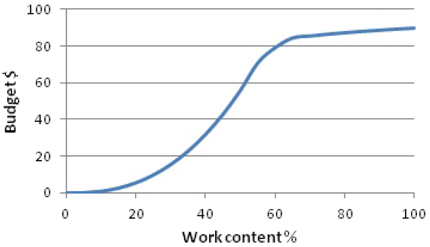
As pointed out earlier, to provide more accurate performance measures there is a need to decouple schedule and cost dimensions. This motivated the partition of the differences between the budget, the PV and the actual costs into cost variance (CV) and schedule variance (SV). This partitioning of the variances into distinct parts is similar to statistical analysis of variance - ANOVA (e.g., [4]). Originally in the EVM and in the ES [8], the values of the PV, EV, ES and AC at each review point are derived from graphs where the PV, EV and AC, are plotted, in monetary terms, against time. In the ED method [6], a couple of graphs are used: Costs against time for the PV and AC and another graph to derive the earned duration. In this second graph, both axes are in time units and the progress, in terms of work content which is measured in time, is drawn against the chronological time. Here, an alternative approach for the derivation of the EV is proposed. The EV assigns a monetary value to work content. Hence, it is proposed to add a third graph in which the cumulative budget is drawn against work content, as in Figure 2 below, and to derive the EV from this graph.

The engineering approach to analyzing cost variances

Recall the partitioning of the project's activity at each review points into three groups: a) Activities which have already been completed, b) Activities which have not yet started and c) Ongoing activities. The actual costs at completion of activities in group (a) are already known and will not be changed. Similarly known are the actual costs of the completed portions of the activities in group (c). Only the actual costs of the activities in group (b) and of the work remain of the activities in group (c) are yet to be determined, and only these costs offer opportunities to reduce cost overruns.

To illustrate, consider, again, the project in [13], which has been reviewed at the end of the 18th period. At this review point, the project's monetary values are: EV = 65 and AC = 83. That is about 27.7% overrun. The activities' partitioning is: (a) = {1, 2, 4, 5, 6}, (b) = {10} and (c) = {3, 7, 8, 9}. Breaking the monetary control data accordingly, EVa = 34, ACa = 48, EVc = 31, while ACc = 35. The costs overrun in group (a) is higher than 41% while that of group (c) is less the 13%. The EAC of activities 1-9 by the project's factor (1.277) is 112.37 but if the overrun factor of group (c) (1.129) is applied, the EAC of this group is a bit less than 61. Hence, the EAC of activities 1-9 is less than 61 + 48 = 109. More information is needed for estimations for activity 10.

It should be noted, however, that as the project progresses onward the project's work remain, which is composed of the activities in groups (b) and (c), decreases. Consequently, opportunities to reduce overruns diminish.

Moreover, the integration of the control effort with the WBS and the OBS - breaking down the control data in accordance to these BSs is not less suitable with regard to cost than it is with regard to time. In fact, the need for this integration was observed (e.g, [22]) in this regard - costs, and there is a cost breakdown structure (CBS), too.

Time related costs: Direct overhead/level of effort

Following the line of distinctions, observe that even the costs of a single activity often include, in addition to components which are expended on the basis of progress; e.g., materials, energy, etc., additional components; e.g., wages, which are paid on the basis of time. A prominent example is the level of effort, or direct overhead (DOH) costs, which is charged "per unit time until the project is completed." [2] (page 546).

"Level of Effort (LoE) is defined as being of a general or supportive nature, with no measurable output, product, or activities; for which the attempt to measure progress discretely or through apportionment is not practicable." "Purpose of guideline: To ensure level of effort (LoE) is limited only to those activities that should not or cannot be discretely planned. Classification of work scope as LoE is limited to activities that have no practicable, measurable output or product associated with technical effort that can be discretely planned and objectively measured at the work package level. Management Value: In every program, there are tasks accomplished that, by their nature, are not measurable. Prudent use of LoE is necessary to minimize the distortion of performance data for effective program management" [14]. These quotes from the DoD-EVM guide reflect the inconvenience of this guide with the LoE. The ANSI EVM standard [16] holds similar attitude and Fleming and Koppelman [15] (page 94) clearly state that LoE is "not recommended for use".

As costs are decoupled from time, these different cost components should also be handled separately. There are the, so-called, direct costs, which depend on work progress and the 'time-related cost'; e.g., LoE and DOH. The definition of the time-related costs is extended: more than a single cost component of this type and with shorter lifespan can be handle, provided the endpoints of the lifespan of each component are defined by definite events; e.g., project's milestones. Further, time-related cost components might be included in the cost of 'regular' activities as well. To handle time-related costs, however, time and costs are re-integrated, as follows.

a) Update direct costs' ETC and EAC by the EVM.

b) Use the duration estimations provided by step 3 of the EPC to estimate the lifespan of each time related cost component.

c) Update the cost estimation of each of these cost components, accordingly.

In certain cases, the present method yields similar results to the 'adjusted' method of [2].

The cost performance index

"In general, EVM and its derivatives use positive values to represent favorable signs of progress and negative values as unfavorable signs." The cost variance is: CV = EV-AC. "Hence, a negative value points out that the project has spent more for the executed activities than what it is worth. To the contrary, a positive value indicates that the project has spent less to gain the value of the executed work." The schedule variance is SV = EV-PV and "similar to CV, a negative SV means that the project is behind the planned schedule, whereas a positive SV represents a project that is ahead of schedule" [6].

There is, however, a fundamental difference between both variances, in that performance is evaluated reversely: Negative CV means cost overrun - more was spent, while negative SV implies that less than planned has been accomplished. Consequently, while the same rule can be applied to both variances, when it comes to indices, there are differences. The schedule indices are: EV/PV, ES/AD and ED/AD (or TED/ TPD) for the EVM, ESM and EDM, respectively, and in all, an index value smaller than one, logically indicates lagging behind schedule. With regard to the cost index, CI = EV/AC, there are, at least, two reservations. First, the EV is the baseline for comparison which should, hence be in the denominator, as in the schedule indices. Second, is it logical that the actual cost are higher than the earned value, that is the project's cost overruns the budget and yet CI < 1? What is, for example, the meaning of CI = 0.783 (= 1/1.277), in the discussion in Section 6.2? This issue has already been noted. "Perhaps one of the more interesting and unexplainable phenomena that emerged in the using of new terminology for C/SCSC (the precursor of EVM) was in the deliberate avoidance of ever using the dreaded word "overrun" in discussions. Interestingly, the management of cost overruns was perhaps the primary reason why EV was required on projects in the first place." [15].

Fortunately, there are others who see it and use the reciprocal term: CI = AC/EV (e.g., [2], page 755), which is much more reasonable. Hopefully, this work will initiate a change in this regard among the PM community.

Summary

The initial motivation for this study was to find a proper way to adjust the time dependent costs: LoE or DOH, according to changes in the performance. The separate handling as proposed in Section 6.3. is rather straightforward but it required means to estimate durations of partial segments of the project. The search in the literature for this kind of estimations, provided no satisfactory answer and a need for a different approach became apparent. The outcome is the proposed engineering project control. A summary of the characterizing features of the EPC and their consequent advantages is provided in Table 3.

As it turned out, the solution for time dependent costs became a byproduct since the EPC offers more than that and more than accurate durations' EAC. It is a practical approach as current computing and information technology enables and facilitates application of all its components and if properly implemented and used, the EPC can improve project control in the broader senses.

Acknowledgement

This study has not been funded in any way, nor there is any other conflict of interests to be reported.

---

References

- Willems LL, Vanhoucke M (2015) Classification of articles and journals on project control and earned value management. International Journal of Project Management 33: 1610-1634.
- Shtub A, Bard JF, Globerson S (2005) Project management: Processes, methodologies and economics. (2nd edn), Prentice Hall, NJ, USA.
- Lin L, Müller R, Zhu F, Liu H (2019) Choosing suitable project control modes to improve the knowledge integration under different uncertainties. International Journal of Project Management 37: 896-911.
- Walpole RE, Myers HM (2012) Probability and statistics for engineers and scientists. (9th edn), Pearson, UK.
- Li C-L, Zhong W (2018) Task scheduling with progress control. IISE Transactions 50: 54-61.
- Khamooshi H, Golafshani H (2014) EDM: Earned duration management, a new approach to schedule performance management and measurement. International Journal of Project Management 32: 1019-1041.
- Anbari FT (2003) Earned value project management method and extensions. Project Management Journal 34: 12-23.
- Lipke W (2003) Schedule is different. Measurable News 31: 31-34.
- Urgilés P, Claver J, Sebastián MA (2019) Analysis of the earned value management and earned schedule techniques in complex hydroelectric power production projects: Cost and time forecast. Complexity 2019: 3190830.
- Pellerin R, Perrier N (2019) A review of methods, techniques and tools for project planning and control. International Journal of Production Research 57: 2160-2178.
- Anisulrahman N, Elshannaway A (2019) Review of earned value management (EVM) methodology, its limitations, and applicable extensions. Journal of Management & Engineering Integration 12: 59-70.
- Goldratt EM (1997) Critical Chain. North River Press.
- Andred PA, Martens A, Vanhoucke M (2019) Using real project schedule data to compare earned schedule and earned duration management project time forecasting capabilities. Automation in Construction 99: 68-78.
- http://acqnotes.com/acqnote/tasks/dod-earned-value-management-guide
- Fleming QW, Koppelman JM (2005) Earned value project management. (3rd edn), Project Management Institute, Inc., PA, USA.
- ANSI (1998) ANSI EIA-748 Standard - Earned value management systems.
- Zhang JY, Wang SJ (2013) The application of earned value management in small and medium-sized hydropower stations project. Applied Mechanics and Materials 357-360: 2371-2378.
- Bryde D, Unterhitzenberger C, Joby R (2018) Conditions of success for earned value analysis in projects. International Journal of Project Management 36: 474-484.
- Nahmias S (2013) Production and operations analysis. McGraw-Hill/Irwin, USA.
- Bolton W (2015) Instrumentation and control systems. (2nd edn), Newnes, UK.
- Koontz H, Odonnell C (1955) Principles of management: An analysis of managerial functions. McGraw-Hill, Inc., NY, USA.
- Kerzner H (2013) Project management: A systems approach to planning, scheduling, and controlling. (11th edn), John Wiley & Sons, Inc., NJ, USA.
Author Details
Moshe Eben-Chaime*
Department of Industrial Engineering & Management, Ben-Gurion University, Israel
Corresponding author
Moshe Eben-Chaime, Department of Industrial Engineering & Management, Ben-Gurion University, Israel.