
International Journal of Industrial and Operations Research
(ISSN: 2633-8947)
Volume 5, Issue 1
Research Article
DOI: 10.35840/2633-8947/6514

Article Formats
A Discussion on the Phase I Screening Robust Estimation Method for Normal Samples
Table of Content
Figures
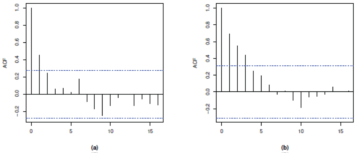
Figure 1: Autocorrelation function of...
Autocorrelation function of the EWMA statistic with λI = 0.6 for (a) a simulated set of k = 50 normal samples of size n = 5 and (b) the piston rings example in Montgomery (2013, 260).
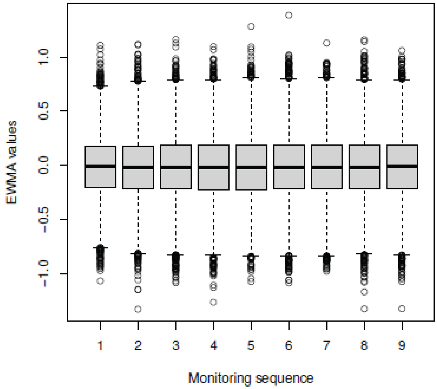
Figure 2: Approximated marginal distribution....
Approximated marginal distribution of the EWMA statistic with λI = 0.6 obtained from 50000 sets of k = 50 normal samples of size n = 5 for the first nine monitoring moments.
Tables
Table 1: Approximated marginal distribution of the EWMA statistic with λI = 0.6 obtained from 50000 sets of k = 50 normal samples of size n = 5 at each monitoring moment t.
Table 2: Control limits for the Phase I EWMA chart with λI = 0.6 obtained from 50000 sets of k = 50 normal samples of size n = 5 for both the formulations of the ESEM.
Table 3: Approximated performance of the Phase I EWMA chart with λI = 0.6 obtained from randomly generated sets of k = 50 normal samples of size n for both the formulations of the ESEM and a nominal 1% FAR level.
References
- Jensen WA, Jones-Farmer LA, Champ CW, Woodall WH (2006) Effects of parameter estimation on control charts properties: A literature review. Journal of Quality Technology 38: 349-364.
- Chakraborti S, Human S, Graham MA (2009) Phase I statistical process control charts: An overview and some results. Quality Engineering 21: 52-62.
- Jones-Farmer LA, Woodall HW, Steiner SH, Champ CW (2014) An overview of Phase I analysis for process improvement and monitoring. Journal of Quality Technology 46: 265-280.
- Zwetsloot I, Schoonhoven S, Does R (2014) A robust estimator for location in Phase I based on an EWMA chart. Journal of Quality Technology 46: 302-316.
- Shen X, Zou C, Jiang W, Tsung F (2013) Monitoring Poisson count data with probability control limits when sample sizes are time varying. Naval Research Logistics 60: 625-636.
- Montgomery D (2013) Introduction to statistical quality control. (7 th edn). John Wiley and Sons, Inc, New York.
- Hillier FS (1969) X and R chart control limits based on a small number of subgroups. Journal of Quality Technology 1: 17-26.
- Yang CH, Hillier FS (1970) Mean and variance control chart limits based on a small number of subgroups. Journal of Quality Technology 2: 9-16.
- King EP (1954) Probability limits for the average chart when process standards are unspecified. Industrial Quality Control 10: 62-64.
- Tatum L (1997) Robust estimation of the process standard deviation for control charts. Technometrics 39: 127-141.
- Schoonhoven M, Riaz M, Does M (2011) Design and analysis of control charts for standard deviation with estimated parameters. Journal of Quality Technology 43: 307-333.
Author Details
CA Panza1*, VH Morales2 and MA Caro3
1Department of Statistics, Universidad Nacional de Colombia, Bogotá, Colombia
2Department of Mathematics and Statistics, Universidad de Córdoba, Montería, Colombia
3Department of Mathematics, Universidad del Atlántico, Barranquilla, Colombia
Corresponding author
CA Panza, Department of Statistics, Universidad Nacional de Colombia, Ciudad Universitaria, Bogotá, Postal Code 111321, Colombia.
Accepted: November 15, 2022 | Published Online: November 17, 2022
Citation: Panza CA, Morales VH, Caro MA (2022) A Discussion on the Phase I Screening Robust Estimation Method for Normal Samples. Int J Ind Operations Res 5:014.
Copyright: © 2022 Panza CA, et al. This is an open-access article distributed under the terms of the Creative Commons Attribution License, which permits unrestricted use, distribution, and reproduction in any medium, provided the original author and source are credited.
Abstract
The screening robust estimation method for Phase I analysis is reviewed. Special attention is devoted to the exponentially weighted moving averages (EWMA) chart that is used in the retrospective stage of monitoring. The central point of the discussion lies in the way the decision threshold of the control procedure is set. Instead of proposing a presumably better Phase I control methodology, the article just aims to show that the aforementioned control chart was not designed in the most accurate form. However, it is shown throughout simulations that the appealing properties of an existing Phase II control procedure can be adapted in order to improve the design of the Phase I EWMA chart used in the robust estimation method for monitoring normal processes.
Keywords
Control charts, Exponentially weighted moving averages (EWMA), Normal distribution, Phase I and II, Process monitoring, Robust estimation
Introduction
In the current practice of the statistical process control (SPC), control schemes have been shown to be an effective tool for assessing the quality level of production processes and service operations. It is well known that control charts can be implemented in both the retrospective (Phase I) and prospective (Phase II) stages of monitoring. A Phase I analysis often involves an exploratory aspect consisting of the applications of statistical methods and techniques in order to better understand the nature of process performance and variation patterns. Once the stability of a process is established by investigating available data for unusual measurements, an appropriate model is selected and estimated from the remaining data. The main goal in Phase I monitoring is to detect drops in the assumed stable model as soon as possible.
A Phase I analysis should include some wider aspects rather than simply designing a control scheme for establishing the stability of the available data. The effectiveness of the on-line process monitoring strongly depends on the success of a well carried out retrospective stage of analysis. Several authors have addressed the need of setting accurate control limits in both the retrospective and the prospective stages of monitoring. Jensen, et al. [1] present an overview about the effect of parameter estimation on the performance of Phase II control char. Chakraborti, et al. [2] provide a detailed review with important technical insights on how to set control limits of univariate control charts in Phase I. Jones-Farmer, et al. [3] present a less technical review that considers chart designing issues and other Phase I methods for univariate and multivariate processes, including profile monitoring, and identifies potential opportunities for further research on Phase I methodologies.
In this article, the screening robust estimation method proposed by Zwetsloot, et al. [4] is reviewed and discussed. The screening robust estimation method was first proposed to be appropriate to deal with several data anomalies in Phase I and aims to overcome the need of developing new control procedures that use robust estimators of the parameters of interest suggested in Jones-Farmer, et al. [3]. The screening robust estimation method involves the novelty idea of using EWMA schemes in Phase I as well. Nevertheless, as will be shown, the decision threshold of the proposed EWMA chart is based on the less recommended criterion as ignores the basic problem of Phase I monitoring.
To show our point of view, it is proposed to adapt the simulation-based algorithm by Shen, et al. [5] in order to reset the control limits of the EWMA chart in Zwetsloot's method. It is thought that the appealing properties of the Phase II EWMA control scheme with probability limits, first introduced by Shen, et al. [5], can also lead to a more accurate way of setting the control limits of the Phase I Zwetloot's EWMA control procedure.
Some General Features of Phase I Analysis
In the following, some relevant issues treated in Chakraborti, et al. [2] will be addressed as they constitute the fundament of this discussion. According to these authors, in the retrospective stage of monitoring, practitioners are faced to a decision problem similar to that of testing the homogeneity of a finite number of data groups.
Let k > 1 denote the amount of independent samples of size n > 1, taken from a some continuous quality characteristic X, whose distribution is parametrized by the vector of p unknown constants. A control scheme consists of the charting statistics Ct, t = 1,2,...,k, and some estimated lower and upper control limits ( and , respectively) being known functions of an estimate of the vector . The plot of all the Ct values together with the estimated control limits form a Phase I control chart. The whole iterative trial-and-error Phase I control procedure is described in Montgomery [6].
The chart signals indicating a possible out-of-control situation as at least one value of the charting statistics lies beyond the most recently calculated control limits. Chakraborti, et al. [2] mainly identify two ways for setting up the control limits and in Phase I. The first way, due to Hillier [7] and Yang and Hillier [8], draws chart limits by controlling the probability of a false alarm for each of the available samples at a desired level. This probability is often referred to as the false alarm rate (FAR). The FAR - criterion approach just requires the knowledge of the marginal distribution of the t-th charting statistic and treats it as if it were statistically independent from those of the rest of the monitoring statistics. That is, the FAR approach does not deal with the simultaneous comparisons of several data subgroups to the same control limits and, consequently, has been proved to severely increase the nominal fixed level.
In the other hand, the second way proposes to evaluate the control limits for a previously specified false alarm probability (FAP), defined as the overall probability of at least one false alarm among the available k subgroups of data. As this approach does not ignore the essential problem of Phase I monitoring, the calculation of the FAP i clearly involves the derivation of the joint probability density function of the charting statistics when the process is in control and the subsequent calculation of the control limits. The FAP criterion was first proposed by King [9] and has turn out to be the most usually recommended way for chart designing in Phase I.
The EWMA-Based Screening Robust Estimation Method (ESEM)
Let Xit denote the i-th, i = 1,...n, observation of the t-th, sample. It is assumed that all the Xit observations are independently and identically normally distributed with mean µ and standard deviation σ when the process is stable. Throughout the respective study, it was set k = 50 and n = 5 or 10.
Zwetsloot, et al. [4] studied some robust estimation methods of the normal location parameter µ along with the efficient estimator for Phase I analysis. They paid special attention to screening methods based on the conventional formulation of the EWMA statistic. These authors recommend the use of a Phase I EWMA chart with λI = 0.6 (or a similar intermediate value) based on a robust estimator of the location parameter, rather than the based on the efficient one for monitoring the mean level.
The Phase I EWMA-based screening robust estimation procedure has to be applied as follows. First, initial robust estimates of the mean and the standard deviation, and , respectively, need to be obtained. The choice of these estimates is presented a little later. Next, for the t-th, t = 1,...,k, sampling moment the Phase I EWMA charting statistic is set to be
with control limits given by
Where and is the smoothing constant for the EWMA statistic in Phase I. When Zt falls beyond the control limits for a given monitoring moment t, due to an assignable cause, the corresponding sample is identified as unacceptable and deleted from the analysis.
Zwetsloot, et al. [4] proposed initially estimate the normal by the median of the averages of the available k samples. This is . This estimator was found out to be efficient and robust to various patterns of outliers. The initial process standard deviation estimator was proposed to be a variant of the biweight estimator proposed by Tatum [10] that is well known for its robustness. The estimation procedure is presented in Tatum [10] and was implemented as set out in Schoonhoven, et al. [11] with normalizing constants d = 1.068 for n = 5 and d = 0.962 for n = 10.
Another key moment in chart designing, is the choice of the constant L in (2). Corresponding L values were proposed to be obtained via simulation by following the recommendations in Chakraborti, et al. [2]. As stated and reported in Zwetsloot, et al. [4], needed L values were computed for all possible combinations of smoothing constants λI = 0.2, 0.6 and 1.0 and sample sizes n = 5 and 10 in the case of standard normal observations. Proposed screening methods were calibrated to reach a nominal 1% FAR.
Critique of the ESEM
The main critique of the ESEM lies on the way the control limits are said to be found. Once the robust estimates for the normal mean and standard deviation are assessed, the ESEM aims to find the value of the constant L in (2) satisfying the recommendations in Chakraborti, et al. [2]. However, the ESEM proponents make no statements about which of those recommendations they exactly followed and even less explain how were implemented.
Although the recommendations in Chakraborti, et al. [2] exhibit a general character, provided relevant insights related to Shewhart-type schemes were only of concern. Recall that the EWMA-based chart is a sequential sampling monitoring scheme and may simply not meet the stochastic independence assumption required by the FAR criterion for Phase I charting design. The use of a Phase I EWMA-based monitoring method faces a problem involving more complex dependence structures than Phase I Shewhart-type schemes do: One due to simultaneous comparisons of multiple samples to the same control limits and another due to the sequential dependence of the monitoring statistics among themselves.
While preparing this paper, it did not take too long to realize that during the implementation of the ESEM via simulation, sets of k = 50 samples from the standardized normal distribution were frequently obtained, for which the respective autocorrelation functions (ACF) were very similar to the one presented in Figure 1a. The ACF for the piston rings example provided in Montgomery [6, 260] is presented in Figure 1b. In other words, both the presented ACF evidence the presence of at least a statistically significant first order autocorrelation pattern. Even so, if the autocorrelation pattern among the EWMA statistics were negligible, the essential problem of Phase I monitoring would still be without addressing. Whichever way Chakraborti's recommendations were implemented, the chosen one leads to the comparison of k = 50 initial samples against a single control region (Figure 1).
In this regard, it would have been more suitable for the ESEM to design an appropriate charting methodology based on the joint multivariate density probability function of the charting EWMA-type statistics Zt, t = 1,...,k, in order to satisfy the FAP designing criterion. Understandably, the deduction of this function could not be an easy task. Following the suggestions in Chakraborti, et al. [2], it may be preferable to work with the marginal conditional distribution of the EWMA statistic at each monitoring moment. As will be seen, this can be achieved by introducing the use of an adapted version of the EWMA chart with probability limits proposed by Shen, et al. [5] in the ESEM.
An EWMA Chart with Probability Limits for Retrospective Analysis
Shen, et al. [5] discuss two computational procedures for determining the upper control limit of an EWMA-type statistic Zt that is effective for monitoring Poisson count data with time-varying sample sizes in Phase II. This scheme is referred to as the EWMAG control chart because has the appealing property of having approximately geometric-distributed run lengths. This implies that the marginal distribution of a single conventional EWMA statistic does not practically depend on the monitoring moment.
According to Shen, et al. [5], at the t-th, t = 1,2..., monitoring moment, the upper control limit ht of the EWMAG has to satisfy the condition
Where α is the desired FAR level.
If it is assumed n
Note that expression (4) is conveniently defined in terms of a desired FAR value. Thus, operatively for our interests, the upper and lower control limits of the proposed monitoring method are evaluated as the and the percentiles, respectively, of the EWMA statistic (1) at the t-th monitoring moment. A simulation-based procedure is summarized below:
• Step 1. Provided that at a given t-th, t = 2,...,k , monitoring moment if there is no out-of-control signal at moment t-1, a large enough number M of values of the "pseudo-EWMA" are computed by generating random samples of size n from and using expression (1). The values and are the initial robust estimates of the normal parameters µ and σ, respectively, proposed by Zwetsloot, et al. [5]. Each of the values are based on a randomly chosen value from the in-control marginal distribution of the EWMA statistic (1) obtained in the preceding monitoring moment t-1. For t = 1, it is assumed . Otherwise, is set as indicates in Step 4.
• Step 2. The and empirical quantiles of the M values of , where α is the desired FAR level, are estimates of the upper and lower control limits, and , respectively, at each monitoring moment t.
• Step 3. The actual current value of is evaluated on the base of the observed data at moment and compared with the respective estimated control limits. If the condition holds, the monitoring is continued to the next moment. Otherwise, the sample corresponding to Zt has to be deleted from the Phase I analysis.
• Step 4. If it is decided to continue, the values of from both the upper and lower tails of the marginal distribution obtained at moment t are eliminated. From the remaining values, one is randomly picked as the preceding value for and the algorithm is restarted.
In few words, the above described approach would avoid the use of the multivariate joint distribution of the k charting EWMA statistics to compute the control limits for the screening procedure. Instead, it aims to approximate them as certain quantiles of the marginal distribution of the EWMA statistic at every monitoring moment t = 1,...,k given that it was possible to establish that the process operates under stable conditions in the immediately preceding moment t-1.
As stated, the proposed screening scheme was calibrated to reach a desired nominal FAR level just to fulfil the purposes of this discussion. If is needed, a more accurate FAP-based charting design can be achieved by following the recommendations of Chakraborti, et al. [2] for FAP-based methods.
Simulation Study
Simulation settings
For comparing both the conventional and the probability limits formulations of the EWMA statistic in the ESEM, the simulation settings were assumed to be the same as in Zwetsloot, et al. [4]. Sets of k = 50 independent random samples of sizes n = 5 or 10 were generated from a normally distributed process with mean µ and standard deviation σ.
The values of the smoothing constant λI for both of the ESEM formulations are chosen to be 0.2, 0.6 and 1.0 for the same reasons outlined in Zwetsloot, et al. [4]. Each charting scheme was calibrated to reach FAR = 1%, so the respective L values for the conventional formulation (1) are those reported in Table 1 by Zwetsloot, et al. [4] for the estimator of the normal process mean µ and the explored k and n values.
Scenarios of interest
As established, needed stable Phase I samples come from a normal distribution with mean µ and standard deviation σ. It is assumed that contaminated observations come from a shifted normal distribution with mean . This is, out-of-control situations are only due to changes in the process mean but not in the standard deviation.
As in Zwetsloot, et al. [4], both the scattered and sustained special causes of variation were considered. So the localized, diffuse, single and multiple step shifting patterns were of interest. For more details on how to deal with the investigated shifting patterns in order to plan current increases in the mean of the studied processes, the reader is asked to consult Section 3.1 in Zwetsloot, et al. [4]. The performance of both the formulations of the ESEM was evaluated for all considered shifting patterns, where δ = 0.0, 0.4, 1.0, 1.6 and 2.0. The in-control state is obtained for δ = 0. As in Zwetsloot, et al. [4], it is assumed µ = 0 and σ = 1, without loss of generality.
Performance evaluation
In practice, Phase I is frequently used as an alternative way for exploratory analysis. Zwetsloot, et al. [4] propose to establish the effectiveness of the Phase I study in terms of both the true-alarm percentage (TAPt) and the false-alarm percentage (FAPt) defined as
Where r denotes the r-th simulation run. For this study, it is set R = 10000. The TAPt and the FAPt were evaluated for all considered shifting patterns in both the formulations of the ESEM.
Some results
For each explored combination of λI and n values, the marginal distribution of the EWMA statistic at the t-th monitoring moment in the Shen's probability limits formulation was approximated by generating M = 50000 "pseudo-EWMA" values as indicated in the first step of the algorithm provided above. In the following, some interesting findings of the carried-out simulations are addressed.
For each monitoring moment, sets of k = 50 random samples of size n were generated from the standardized normal distribution in order to obtain the marginal distribution of the EWMA statistic. Table 1 shows the main numeric attributes of the estimated marginal distribution with λI = 0.6 and n = 5. There are presented the estimated quartiles (Q0.25, Q0.50 and Q0.75), the mean and standard deviation of each distribution for the first six and the last monitoring moments.
It should be noted that, except for the first two monitoring moments, the marginal distribution of the EWMA statistic remains practically invariant. It could even be said that the marginal distribution of the first two moments are not so different from those obtained for further moments. This fact can be better appreciated in Figure 2, where the approximated marginal distributions of the first nine monitoring moments are shown (Figure 2).
The aforementioned fact has the natural consequence of drawing the approximately same control limits at each monitoring moment. In passing, it was stated in Chakraborti, et al. [2] that a commonly used approach to establish chart limits is to control the FAR at a desired level at every monitoring moment. This approach just requires the knowledge of the in-control marginal distribution for the t-th charting statistic, which is typically the same for all t = 1,...k, so the FAR is the same for all available samples. This is clearly the case the adapted version of Shen's procedure is dealing with. When FAR = 0.01, the results reported in Table 2 are obtained.
In Table 2, there are shown the estimated lower and upper control limits of the ESEM calculated on five sets of k = 5 independent samples of size n = 5 randomly generated from the standardized normal distribution. Each pair of control limits were computed for both the conventional and the probability limits formulations of the EWMA statistic with λI = 0.6. According to the results reported in Table 1, 50 UCL values that are very similar to each other should be expected for the probability limits formulation. So should be the LCL values. In Table 2, there are reported the maximum and the minimum of all the observed values for each set of samples as the respective upper and lower control limits of the adapted Shen's formulation. It has to be noted that the control limits calculated by both the methodologies are approximately the same for each set of samples. However, the ones calculated by the probability limits formulation are always slightly narrower.
Although the respective results are not reported, similar conclusions to those presented were reached for the other explored λI values with n = 5 and for all λI values in combination with n = 10.
Moreover, the detection abilities for both the formulations of the ESEM were estimated by using formulae (5) and (6) for each proposed out-of-control scenario. The probabilities of the conventional formulation of the ESEM were recreated for the location robust estimator and the same out-of-control scenarios and values proposed in Zwetsloot, et al. [4]. The results for λI = 0.6 are provided in Table 3.
It can be seen that, except for some reported cases, the Phase I EWMA chart performance of Zwetsloot's proposal exhibits slightly smaller TAP values than that of the Shen's probability limits formulation. This is not an unexpected result as the carried-out simulations suggest a narrower decision threshold for the probability limits formulation of the EWMA chart. The FAP values for both the formulations are comparable in all explored cases. Similar results were obtained for the other set values of the smoothing constant λI and the same estimators of the process parameters.
Recall that the probability limits formulation was intentionally calibrated to satisfy the FAR criterion of chart designing. Whatever it was, the way in which the EWMA chart of the ESEM was initially conceived gave it a performance that is quite similar to that of a FAR-based control methodology. However, the mere dependent nature of the EWMA statistic prevents chart designing in Phase I from being based on the FAR criterion because it requires the stochastic independence of the monitoring statistics.
Concluding Remarks and Recommendations
As was initially thought, the EWMA chart in the ESEM is conceptually a Phase I monitoring procedure whose performance closely resembles that of FAR-based methods. It is well known that the FAR is the least recommended criterion for chart designing since it ignores the fundamental problem of Phase I monitoring consisting of simultaneous comparisons of multiple data groups against the same control limits. However, the ESEM makes a significant contribution in the search and implementation of new methodologies for Phase I retrospective analysis providing relevant insights about the robust parameter estimation in normally distributed processes.
On the other hand, we feel that it is possible to use the appealing distributional properties of the EWMAG chart with probability limits proposed by Shen, et al. [5] to overcome the disadvantages of the conventional ESEM formulation and to design accurate monitoring proposals for Phase I based on the more suitable FAP criterion. Proposals may even include the use of cumulative sums (CUSUM) monitoring schemes for Phase I. These are topics of our current research work.